the Creative Commons Attribution 4.0 License.
the Creative Commons Attribution 4.0 License.
 | 25 Feb 2020
Earth system data cubes unravel global multivariate dynamics
Miguel D. Mahecha
Fabian Gans
Gunnar Brandt
Rune Christiansen
Sarah E. Cornell
Normann Fomferra
Guido Kraemer
Jonas Peters
Paul Bodesheim
Gustau Camps-Valls
Jonathan F. Donges
Wouter Dorigo
Lina M. Estupinan-Suarez
Victor H. Gutierrez-Velez
Martin Gutwin
Martin Jung
Maria C. Londoño
Diego G. Miralles
Phillip Papastefanou
Markus Reichstein
Understanding Earth system dynamics in light of ongoing human intervention and dependency remains a major scientific challenge. The unprecedented availability of data streams describing different facets of the Earth now offers fundamentally new avenues to address this quest. However, several practical hurdles, especially the lack of data interoperability, limit the joint potential of these data streams. Today, many initiatives within and beyond the Earth system sciences are exploring new approaches to overcome these hurdles and meet the growing interdisciplinary need for data-intensive research; using data cubes is one promising avenue. Here, we introduce the concept of Earth system data cubes and how to operate on them in a formal way. The idea is that treating multiple data dimensions, such as spatial, temporal, variable, frequency, and other grids alike, allows effective application of user-defined functions to co-interpret Earth observations and/or model–data integration. An implementation of this concept combines analysis-ready data cubes with a suitable analytic interface. In three case studies, we demonstrate how the concept and its implementation facilitate the execution of complex workflows for research across multiple variables, and spatial and temporal scales: (1) summary statistics for ecosystem and climate dynamics; (2) intrinsic dimensionality analysis on multiple timescales; and (3) model–data integration. We discuss the emerging perspectives for investigating global interacting and coupled phenomena in observed or simulated data. In particular, we see many emerging perspectives of this approach for interpreting large-scale model ensembles. The latest developments in machine learning, causal inference, and model–data integration can be seamlessly implemented in the proposed framework, supporting rapid progress in data-intensive research across disciplinary boundaries.
- Article
(8608 KB) - Full-text XML
- BibTeX
- EndNote


Predicting the Earth system's future trajectory given ongoing human intervention into the climate system and land surface transformations requires a deep understanding of its functioning (Schellnhuber, 1999; IPCC, 2013). In particular, it requires unravelling the complex interactions between the Earth's subsystems, often termed as “spheres”: atmosphere, biosphere, hydrosphere (including oceans and cryosphere), pedosphere, or lithosphere, and increasingly the “anthroposphere”. The grand opportunity today is that many key processes in various subsystems of the Earth are constantly monitored. Networks of ecological, hydrometeorological, and atmospheric in situ measurements, for instance, provide continuous insights into the dynamics of the terrestrial water and carbon fluxes (Dorigo et al., 2011; Baldocchi, 2014; Wingate et al., 2015; Mahecha et al., 2017). Earth observations retrieved from satellite remote sensing enable a synoptic view of the planet and describe a wide range of phenomena in space and time (Pfeifer et al., 2012; Skidmore et al., 2015; Mathieu et al., 2017). The subsequent integration of in situ and space-derived data, e.g. via machine learning methods, leads to a range of unprecedented quasi-observational data streams (e.g. Tramontana et al., 2016; Balsamo et al., 2018; Bodesheim et al., 2018; Jung et al., 2019). Likewise, diagnostic models that encode basic process knowledge, but which are essentially driven by observations, produce highly relevant data products (see, e.g. Duveiller and Cescatti, 2016; Jiang and Ryu, 2016a; Martens et al., 2017; Ryu et al., 2018). Many of these derived data streams are essential for monitoring the climate system including land surface dynamics (see, for instance, the essential climate variables, ECVs; Hollmann et al., 2013; Bojinski et al., 2014), oceans at different depths (essential ocean variables, EOVs; Miloslavich et al., 2018), or the various aspects of biodiversity (essential biodiversity variables, EBVs; Pereira et al., 2013). Together, these essential variables describe the state of the planet at a given moment in time and are indispensable for evaluating Earth system models (Eyring et al., 2019).
With regard to the acquisition of sensor measurements and the derivation of downstream data products, Earth system sciences are well prepared. But can this multitude of data streams be used efficiently to diagnose the state of the Earth system? In principle, our answer would be affirmative, but in practical terms we perceive high barriers to interconnecting multiple data streams and further linking these to data analytic frameworks (as discussed for the EBVs by Hardisty et al., 2019). Examples of these issues are (i) insufficient data discoverability, (ii) access barriers, e.g. restrictive data use policies, (iii) lack of capacity building for interpretation, e.g. understanding the assumptions and suitable areas of application, (iv) quality and uncertainty information, (v) persistency of data sets and evolution of maintained data sets, (vi) reproducibility for independent researchers, (vii) inconsistencies in naming or unit conventions, and (viii) co-interpretability, e.g. either due to spatiotemporal alignment issues or physical inconsistencies, among others. Some of these issues are relevant to specific data streams and scientific communities only. In most cases, however, these issues reflect the neglect of the FAIR principles (to be “findable, accessible, interoperable, and re-usable”; Wilkinson et al., 2016). If the lack of FAIR principles and limited (co-)interpretability come together, they constitute a major obstacle in science and slow down the path to new discoveries. Or, to put it as a challenge, we need new solutions that minimize the obstacles that hinder scientists from capitalizing on the existing data streams and accelerate scientific progress. More specifically, we need interfaces that allow for interacting with a wide range of data streams and enable their joint analysis either locally or in the cloud.
As long as we do not overcome data interoperability limitations, Earth system sciences cannot fully exploit the promises of novel data-driven exploration and modelling approaches to answer key questions related to rapid changes in the Earth system (Karpatne et al., 2018; Bergen et al., 2019; Camps-Valls et al., 2019; Reichstein et al., 2019). A variety of approaches have been developed to interpret Earth observations and big data in the Earth system sciences in general (for an overview, see, e.g. Sudmanns et al., 2019) and gridded spatiotemporal data as a special case (Nativi et al., 2017; Lu et al., 2018). For the latter, data cubes have recently become popular, addressing an increasing demand for efficient access, analysis, and processing capabilities for high-resolution remote sensing products. The existing data cube initiatives and concepts (e.g. Baumann et al., 2016; Lewis et al., 2017; Nativi et al., 2017; Appel and Pebesma, 2019; Giuliani et al., 2019) vary in their motivations and functionalities. Most of the data cube initiatives are, however, motivated by the need for accessing singular (very-)high-resolution data cubes, e.g. from satellite remote sensing or climate reanalysis, and not by the need for global multivariate data exploitation.
This paper has two objectives: first, we aim to formalize the idea of an Earth system data cube (ESDC) that is tailored to explore a variety of Earth system data streams together and thus largely complements the existing approaches. The proposed mathematical formalism intends to illustrate how one can efficiently operate such data cubes. Second, the paper aims at introducing the Earth System Data Lab (ESDL; https://earthsystemdatalab.net, last access: 21 February 2020). The ESDL is an integrated data and analytical hub that curates a multitude of data streams representing key processes of the different subsystems of the Earth in a common data model and coordinate reference system. This infrastructure enables researchers to apply their user-defined functions (UDFs) to these analysis-ready data (ARD). Together, these elements minimize the hurdle to co-explore a multitude of Earth system data streams. Most known initiatives intend to preserve the resolutions of the underlying data and facilitate their direct exploitation, like the Earth Server (Baumann et al., 2016) or the Google Earth Engine (Gorelick et al., 2017). The ESDL, instead, is built around singular data cubes on common spatiotemporal grids that include a high number of variables as a dimension in its own right. This design principle is thought to be advantageous compared to building data cubes from individual data streams without considering their interactions from the very beginning. Due to its multivariate structure and the easy-to-use interface, the ESDL is well suited for being part of data-driven challenges, as regularly organized by the machine learning community, for example.
The remainder of the paper is organized as follows: Sect. 2 introduces the concept based on a formal definition of Earth system data cubes and explains how user-defined functions can interact with them. In Sect. 3, we describe the implementation of the Earth System Data Lab in the programming language Julia and as a cloud-based data hub. Section 4 then illustrates three research use cases that highlight different ways to make use of the ESDL. We present an example from an univariate analysis, characterizing seasonal dynamics of some selected variables; an example from high-dimensional data analysis; and an example for the representation of a model–data integration approach. In Sect. 5, we discuss the current advantages and limitations of our approach and put an emphasis on required future developments.
Our vision is that multiple spatiotemporal data streams shall be treated as a singular yet potentially very high-dimensional data stream. We call this singular data stream an Earth system data cube. For the sake of clarity, we introduce a mathematical representation of the Earth system data cube and define operations on it. Further details on an efficient implementation are provided in Sect. 3.2 and 3.3.
Suppose we observe p variables , each under a (possibly different) range of conditions. A first step towards data integration is to (re)sample all data streams onto a common domain J (e.g. a spatiotemporal grid) to obtain the indexed set , …, of multivariate observations. Observations obtained from different variables are then identified as different coordinates in the multivariate array Y. However, when calculating simple variable summaries or performing spatiotemporal aggregations of the data, such a representation can be computationally obstructive. We therefore propose to consider the “variable indicator” k∈{1, …, p} as simply another dimension of the index set and view the data as the collection {Xi}i∈I of univariate observations, where , …, p}1 and where . With this idea in mind, we now formally define the Earth system data cube (“data cube” in short).
A data cube C consists of a triplet (L, G, X) of components to be described below.
-
L is a set of labels, called dimensions, describing the axes of the data cube. For example, L={lat, long, time, var} describes a data cube containing spatiotemporal observations from a range of different variables. The number of dimensions |L| is referred to as the order of cube C; in the above example, |L|=4.
-
G is a collection {grid(ℓ)}ℓ∈L of grids along the axes in L. For every ℓ∈L, the set grid(ℓ) is a discrete subset of the domain of the axis ℓ, specifying the resolution at which data are available along this axis. Every set grid(ℓ) is required to contain at least two elements. Dimensions containing only one grid point are dropped. The collection G defines the hyper-rectangular index set , motivating the name “cube”. For example,
Since G and I(G) are in one-to-one correspondence, we will use the two interchangeably.
-
X is a collection of data observed at the grid points in I(G). Here, “NA” refers to “not available”.
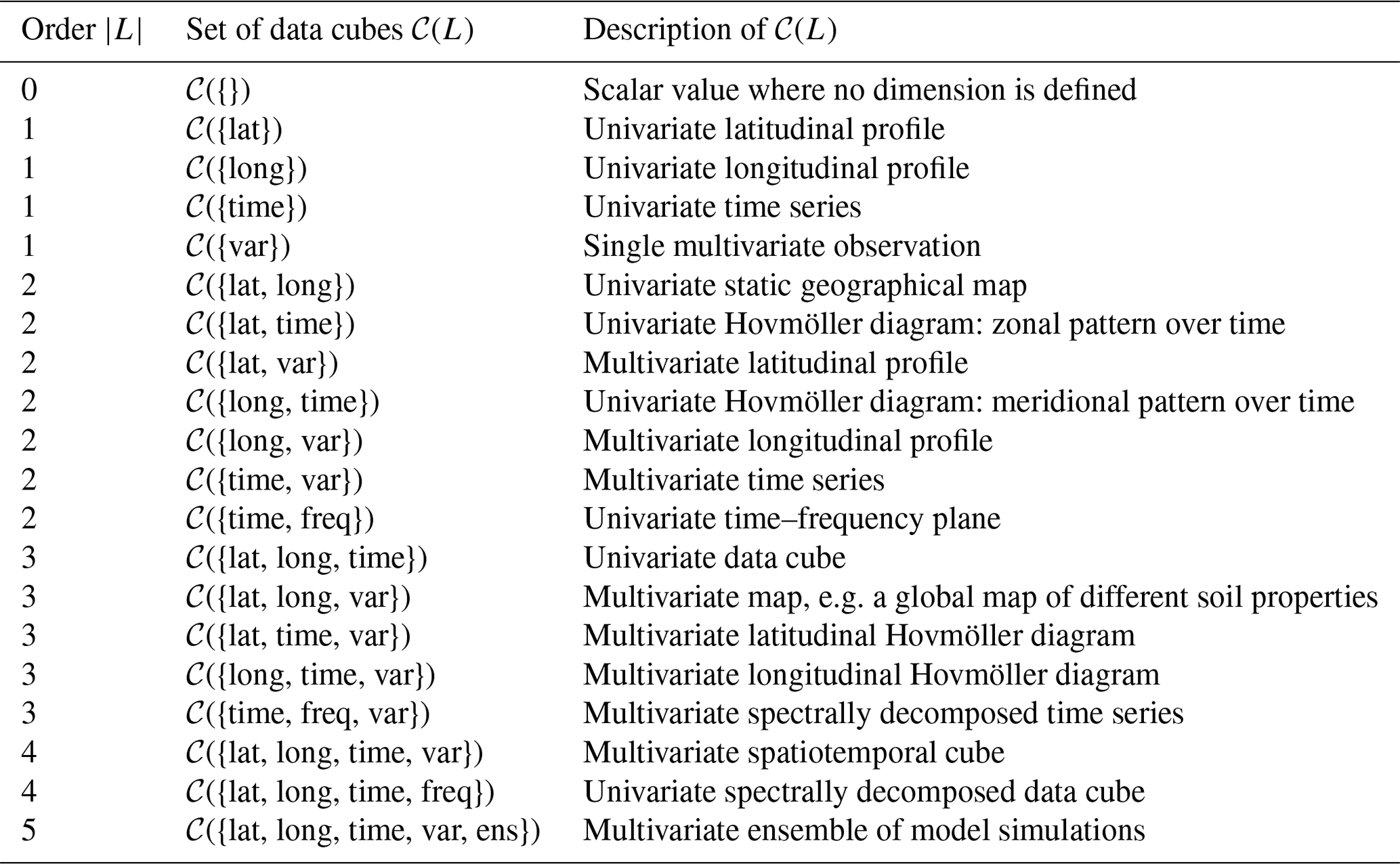
In this view, the data can be treated as a collection {Xi}i∈I(G) of univariate observations, even if they encode different variables. In the above example, the variable axis is a nominal grid with the entries GPP (gross primary production), SWC (soil water content), and Rg (global radiation). The set of all data cubes with dimensions L will be denoted by 𝒞(L). Data cubes that contain one variable only can be considered as special case; other common choices of L are described in Table 1. The list of example axes labels used in the table is, of course, not exhaustive. Other relevant dimensions could be, for example, model versions, model parameters, quality flags, or uncertainty estimates. Note that, by definition, a data cube only depends on its dimensions through the set of axes L and is therefore indifferent to any order of these. In the remainder of this article, the notion of data cubes refers to this concept. Note that dropping dimensions that only contain one grid point is not the only possible way of working with data cubes. Another equally valid idea is to maintain grids of length 1 and integrate them to the workflow.
Table 1Typical sets of data cubes 𝒞(L) of varying orders |L| with characteristic dimensions L.
2.1 Operations on an Earth system data cube
To exploit an Earth system data cube efficiently, scientific workflows need to be translated into operations executable on data cubes as described above. More specifically, the output of each operation on a data cube should yield another data cube. The entire workflow of a project, possibly a succession of analyses performed by different collaborators, can then be expressed as a composition of several UDFs performed on a single (input) data cube. Besides unifying all statistical data analyses into a common concept, the idea of expressing workflows as functional operations on data cubes comes with another important advantage: as soon as a workflow is implemented as a suitable set of UDFs, it can be reused on any other sufficiently similar data cube to produce the same kind of output.
In its most general form, a user-defined function C↦f(C) operates by (i) extracting relevant information from C, (ii) performing calculations on the extracted information, and (iii) storing these calculations into a new data cube f(C). In order to perform step (i), f expects a minimal set of dimensions E of the input cube. The returned set of axes for an input cube with dimensions E will be denoted by R. That is, f is a mapping such that
Alongside the function f, one has to define the sets E and R, which we will refer to as minimal input and minimal output dimensions, respectively.
A major advantage of thinking in data cube workflows is that low-dimensional functions can be applied to higher-dimensional cubes by simple functional extensions: a function can be acting along a particular set of dimensions while looping across all unspecified dimensions. For example, the function that computes the temporal mean of a univariate time series should allow for an input data cube, which, in addition to a temporal grid, contains spatial information. The output of such an operation should then be a cube of spatially gridded temporal means. Similarly, the function should be applicable to cubes containing multivariate observations. Here, we expect the output to contain one temporal mean per supplied variable.
In general, a function f defined on 𝒞(E) should naturally extend to a function from 𝒞(E∪A) to 𝒞(R∪A) with by executing the described “apply” operation. The code package accompanying this paper (described in Sect. 3) automatically equips every UDF with such a functionality. A schematic description of this approach is illustrated in Fig. 1.
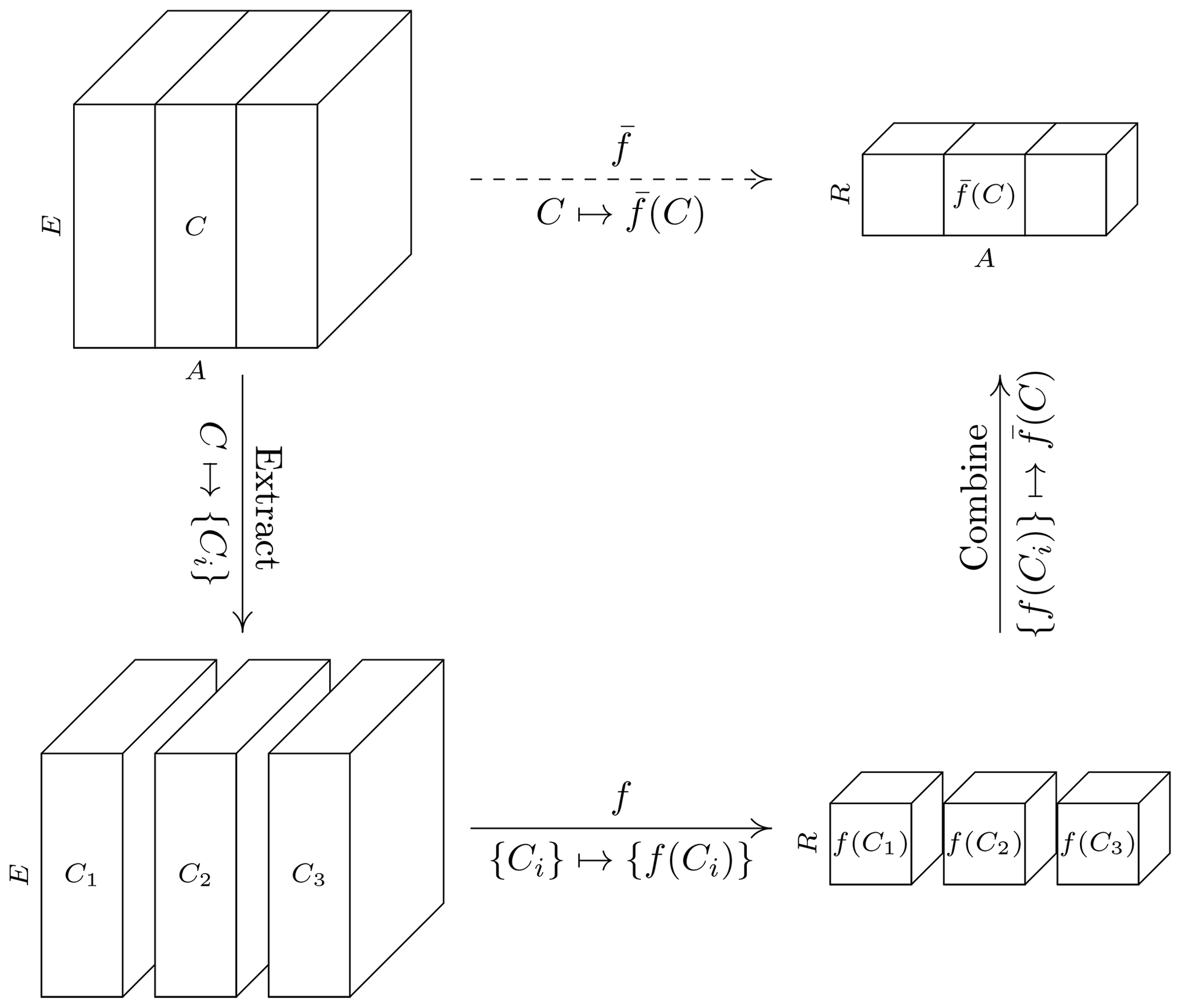
Figure 1Schematic illustration of the “apply” functionality: a function is extended to the set of cubes with dimensions E∪A, where A is an arbitrary set of dimensions with . Given a cube , the extension is constructed by iterating over all grid points i along the dimensions in A to obtain the collection {Ci}⊆𝒞(E) of sliced cubes, applying f to every cube Ci separately, and binding the collection {f(Ci)} into the output cube . Here, the index i runs through all elements in ![]() grid(a).
grid(a).
The approach outlined above is very convenient to describe workflows, i.e. recursive chains of UDFs. Let f1, … fn be a sequence of UDFs with corresponding minimal input/output dimensions (E1, R1), …, (En, Rn). If an output dimension Ri is a subset of subsequent input Ei+1, we can chain these functions. A recursive workflow emerges when for all i, by iteratively chaining f1, …, fn upon one another. The input/output dimensions of the resulting cube are (E1, Rn).
Overall, the definition of an Earth system data cube and associated operations on it do not only guide the implementation strategy but also help us summarize potentially complicated analytic procedures in a common language. For the sake of readability, in the following, we will not distinguish between a function f (defined only for minimal input) and its extension (equipped with the apply functionality; see Fig. 1). The former will be referred to as an “atomic” function. We typically indicate the minimal input/output dimensions (E, R) of a function f by writing . Since the pair (E, R) does not determine the mapping f, this notation should not be understood as the parameterization of a function class but rather provide an easy way to perform input control and to anticipate the output dimensions of a cube returned by f. For instance, following the discussion above, a function denoted by can be applied to any cube with dimension E∪A, satisfying that , and returns a cube with dimensions R∪A. To avoid ambiguities, additional notation is needed when distinguishing between two functions with the same pair of minimal input/output dimensions.
2.2 Examples
In the following, we present some special operations that are routinely needed in explorations of Earth system data cubes:
“Reducing” describes a function that calculates some scalar measure (e.g. the sample mean). Consider, for instance, the need to estimate the mean of a univariate data cube, of course weighted by the area of the spatial grid cells. An operation of this kind expects a cube with dimensions E={lat, long, time} and returns a cube with dimensions R={ } and is therefore a mapping:
This mapping can now be applied to any data cube of potentially higher (but not lower) dimensionality. For instance, f is automatically extended to a multivariate spatiotemporal data cube (Table 1) with the mapping
which computes one spatiotemporal mean for each variable.
“Cropping” is subsetting a data cube while maintaining the order of a cube. A cropping operation typically reduces certain axes of a data cube to only contain specified grid points (and therefore requires the input cube to contain these grid points). For instance, a function that extracts a certain “cropped” fraction T0 along the temporal cover expects an input cube containing a time axis with a grid at least as highly resolved as T0. This function preserves the dimensionality of the cube but reduces the grid along the time axis; i.e.
where we have used 𝒞(L|P) to denote the set of cubes with dimensions L satisfying the condition P. Thanks to the apply functionality, this atomic function can be used on any cube of higher order. For example, it is readily extended to a mapping:
which crops the time axis of cubes with dimensions {lat, long, time}. Analogously, all dimensions can be subsetted as long as the length of the dimension is larger than 1. The latter would be called slicing.
“Slicing” refers to a subsetting operation in which a dimension of the cube is degenerated, and the order of the cube is reduced and can be interpreted as a special form of cropping. For instance, if we only select a singular time instance t0, the time dimension effectively vanishes as we do not longer need a vector-spaced dimension to represent its values. When applied to a spatiotemporal data cube, this amounts to a mapping:
“Expansions” are operations where the order of the output cube is higher than the order of the corresponding input cube. A discrete spectral decomposition of time series, for example, generates a new dimension with characteristic frequency classes:
“Multiple cube handling” is often needed, for instance, when fitting a regression model where response and predictions are stored in different cubes. Also, we may be interested in outputting the fitted values and the residuals in two separate cubes. This amounts to an atomic operation:
which expects a multivariate data cube for the predictors C1∈𝒞({time, var}) and a univariate cube for the targets C2∈𝒞({time}). The output consists of a vector of fitted parameters para}) and a residual time series time}) to compute the model performance. This concept also allows the integration of more than two input and/or output cubes.
The concept as described in Sect. 2 is generic, i.e. independent of the implemented Earth system data cube and of the technical solution of the implementation. Figure 2 shows how the concept outlined above is realized from a practical point of view. The flowchart shows that the starting point is the collection of relevant data streams which then need to be preprocessed in order to be interpretable as a single data cube. The ESDC itself may be stored locally or in the cloud and can be accessed from various users simultaneously based on different application programming interfaces (APIs). In the following, we firstly present the data used in our implementation of the ESDL which is available online, and secondly describe the implementation strategy for the API we developed in this project.
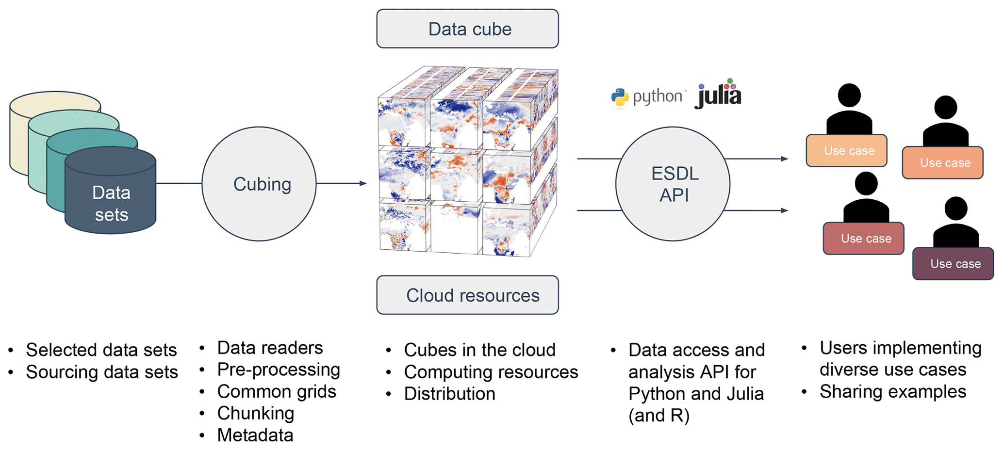
Figure 2Workflow putting the ESDL concept into practice: selected data sets are preprocessed to common grids and saved in cloud-ready data formats (Zarr). Based on these cubed data sets, a global Earth system data cube can be produced that is either stored locally or in the cloud. Via appropriate application programming interfaces (APIs), users can efficiently access the ESDC in their native language. Users can fully focus on designing user-defined functions and workflows.
3.1 Data streams in the ESDL
The data streams included so far were chosen to enable research on the following topics (a complete list is provided in Appendix A):
-
Ecosystem states at the global scale in terms of relevant biophysical variables. Examples are leaf area index (LAI), the fraction of photosynthetically active radiation (fAPAR), and albedo (Disney et al., 2016; Pinty et al., 2006; Blessing and Löw, 2017).
-
Biosphere–atmosphere interactions as encoded in land fluxes of CO2, i.e. GPP, terrestrial ecosystem respiration (Reco), and the net ecosystem exchange (NEE) as well as the latent heat (LE) and sensible heat (H) energy fluxes. Here, we rely mostly on the FLUXCOM data suite (Tramontana et al., 2016; Jung et al., 2019).
-
Terrestrial hydrology requires a wide range of variables. We mainly ingest data from the Global Land Evaporation Amsterdam Model (GLEAM; Martens et al., 2017; Miralles et al., 2011) which provide a series of relevant surface hydrological properties such as surface (SM) and root-zone soil moisture (SMroot) but also potential evaporation (Ep) and evaporative stress (S) conditions, among others. Ingesting entire products such as GLEAM ensures internal consistency.
-
State of the atmosphere is described using data generated by the Climate Change Initiative (CCI) by the European Space Agency (ESA) in terms of aerosol optical depth at different wavelengths (AOD550, AOD555, AOD659, and AOD1610; Holzer-Popp et al., 2013), total ozone column (Van Roozendael et al., 2012; Lerot et al., 2014), as well as surface ozone (which is more relevant to plants), and total column water vapour (TCWV; Schröder et al., 2012; Schneider et al., 2013).
-
Meteorological conditions are described via the reanalysis data, i.e. the ERA5 product. Additionally, precipitation is ingested from the Global Precipitation Climatology Project (GPCP; Adler et al., 2003; Huffman et al., 2009).
Together, these data streams form data cubes of intermediate spatial and temporal resolutions (0.25, 0.083∘; both 8 d), visualized in Fig. 3. The variables described here are described in more detail in a list provided in Appendix A, which may, however, already be incomplete at the time of publication, as the ESDL is a living data suite, constantly expanding according to users' requests. For the latest overview, we refer the reader to the website (https://www.earthsystemdatalab.net/, last access: 21 February 2020). Note that we have not considered the integration of uncertainty as another dimension in the current implementation. The rationale is that each of the data products comes with a specific uncertainty flag or estimate that cannot be merged in an own dimension. This is an open aspect that needs to be addressed in future developments.
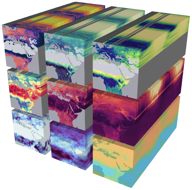
Figure 3Visualization of the implemented Earth system data cube (an animation is provided online at https://youtu.be/9L4-fq48Ev0, last access: 21 February 2020). The figure shows from the top left to bottom right the variables sensible heat (H), latent heat (LE), gross primary production (GPP), surface moisture (SM), land surface temperature (LST), air temperature (Tair), cloudiness (C), precipitation (P), and water vapour (V). References to the individual data sources are given in Appendix A. Here, the resolution in space is 0.25∘ and 8 d in time, and we are inspecting the time from May 2008 to May 2010; the spatial range is from 15∘ S to 60∘ N, and 10∘ E to 65∘ W.
To show the portability of the approach, we have developed a regional data cube for Colombia. This work supports the Colombian Biodiversity Observational Network activities within the Group on Earth Observations Biodiversity Observation Network (GEO BON). This regional data cube has a 1 km (0.083∘) resolution and focuses on remote-sensing-derived data products (i.e. LAI, fAPAR, the normalized difference vegetation index (NDVI), the enhanced vegetation index (EVI), LST, and burnt area). In addition to the global ESDL, monthly mean products such as cloud cover (Wilson and Jetz, 2016) have been ingested given their recurrent applicability in biodiversity studies at regional scales. Data layers from governmental organizations providing detailed information about ecosystems are also available that allow a national characterization and deeper understanding of ecosystem changes by natural or human drivers. These are maps of biotic units (Londoño et al., 2017), wetlands (Flórez et al., 2016), and agriculture frontier maps (MADR-UPRA, 2017). Additionally, GPP, evapotranspiration, shortwave radiation, PAR, and diffuse PAR from the Breathing Earth System Simulator (BESS; Ryu et al., 2011, 2018; Jiang and Ryu, 2016b) and albedo from QA4ECV (http://www.qa4ecv.eu/, last access: 21 February 2020) are available, among others. This regional Earth system data cube should serve as a platform for analysis in a region with variability of landscape, high biodiversity and ecosystem transitions gradients, and facing rapid land use change (Sierra et al., 2017).
3.2 Implementation
To put the concept of an Earth system data cube as outlined in Sect. 2 into practice, we need suitable access APIs (see Fig. 2). A co-author of this paper (FG) developed one API in the relatively young scientific programming language Julia (https://julialang.org/, last access: 21 February 2020; Bezanson et al., 2017) which is provided via the ESDL.jl package. Additionally, all functionalities are also available in Python based on existing libraries and documented online. In both cases, the goal was that the user does not have to explicitly deal with the complexities of sequential data input/output handling and can concentrate on implementing the atomic functions and workflows, while the system takes care of necessary out of core and out-of-memory computations. The following is a sketched description of the principles of the Julia-based ESDL.jl implementation. We chose Julia to translate the concepts outlined into efficient computer code because it has clear advantages for data cube applications besides its general elegance in scientific computing in terms of speed, dynamic programming, multiple dispatch, and syntax (Perkel, 2019). Specifically, Julia allows for generic processing of high-dimensional data without large code repetitions. At the core of the Julia ESDL.jl toolbox are the mapslices and mapCube functions, which execute user-defined functions on the data cube as follows:
-
Given some large data cube C=(L, G, X), the
ESDLfunctionsubsetcube(C) will retrieve a handle to C that fully describes L and G. -
Knowledge of the desired L and G allows us to develop a suitable user-defined function .
-
Depending on the exact needs,
mapslicesandmapCubewill then be used to apply the on a cube as illustrated in Fig. 1.mapCubeis a strict implementation of the cube mapping concept described here, where it is mandatory to explicitly describe E and R such that the atomic function is fully operational.mapslicesis a convenient wrapper around themapCubefunction that tries to impute the output dimensions given the user function definition to ease the application of the functions where the output dimensions are trivial. Internally,mapslicesandmapCubeverify that E⊆L and other conditions.
The case studies developed in Sect. 4 are accompanied by code that illustrates this approach in practice.
Of course there are also alternatives to Julia. Lu et al. (2018) recently reviewed different ways of applying functions on array data sets in R, Octave, Python, Rasdaman, and SciDB. One requirement of such a mapping function is that it should be scalable, which means that it should process data larger than the computer memory and, if needed, in parallel. While existing solutions are sufficient for certain applications, most are not consistent with the cube mapping concept as described in Sect. 2. For instance, the required handling of complex workflows of multiple cubes (Eq. 8) is typically not possible in the existing solutions that have been reviewed. In some cases, issues in the computational efficiency of the underlying programming languages render certain solutions not suitable. This is particularly the case when user-defined functions become complex. Likewise, certain properties such as the desired indifference to the ordering in axes dimensions are often not foreseen. One suitable alternative to Julia is available in Python. The xarray (http://xarray.pydata.org, last access: 21 February 2020) and dask packages have been successfully utilized in the Open Data Cube, Pangeo, and xcube initiatives. Extensive descriptions on how to work in the ESDL with both Python and Julia can be accessed from the following website: https://www.earthsystemdatalab.net/ (last access: 21 February 2020). The open-source implementation of the ESDL also implies that one can easily extend the stored data sets. The online documentation shows in detail how additional data can be added to the ESDL. In particular, if the data share common axes and are stored in a compatible format (as described below in Sect. 3.3), this does not require major efforts.
3.3 Storage and processing of the data cube
The ESDL has been built as a generic tool. It is prepared to handle very large volumes of data. Storage techniques for large raster geodata are generally split into two categories: database-like solutions like Rasdaman (Baumann et al., 1998) or SciDB (Stonebraker et al., 2013) access data directly through file formats that follow metadata conventions like HDF5 (https://www.hdfgroup.org/, last access: 21 February 2020) or NetCDF (https://www.unidata.ucar.edu/software/netcdf/, last access: 21 February 2020). Database solutions shine in settings where multiple users repeatedly request (typically small) subsets of data cube, which might not be rectangular, because the database can accelerate access by adjusting to common access patterns. However, for batch processing large portions of a data cube, every data entry is ideally accessed only once during the whole computation. Hence, when large fractions of some data cube have to be accessed, users will usually avoid the overhead of building and maintaining a database and rather aim for accessing the data directly from their files. This experience is often perceived as more “natural” for Earth system scientists who are used to “touching” their data, knowing where files are located, and so forth. Databases instead offer, by construction, an entry point to an otherwise unknown data set.
One disadvantage of the traditional file formats used for storing gridded data is that their data chunks are contained in single files that may become impossible to handle efficiently. This is not problematic when the data are stored on a regular file system where the file format library can read only parts of the file. In cloud-based storage systems, it is not common to have an API for accessing only parts of an object, so these file formats are not well suited for being stored in the cloud. Recently, novel solutions for this issue were proposed, including modifications to existing storage formats, e.g. HDF5 cloud, or cloud-optimized GeoTiff, among others, as well as completely new storage formats, in particular Zarr (https://zarr.readthedocs.io/, last access: 21 February 2020) and TileDB (https://tiledb.io/, last access: 21 February 2020). While working with these formats is very similar to traditional solutions (like HDF5 and NetCDF), these new formats are optimized for cloud storage as well as for parallel read and write operations. Here, we chose to use the new Zarr format. The reason is that it enables us to share the data cube through an object storage service, where the data are public and can be analysed directly. Python packages for accessing and analysing large N-dimensional data sets like xarray and dask, which make a wide range of existing tools readily usable on the cube, and a Julia approach to read Zarr data have been implemented as well.
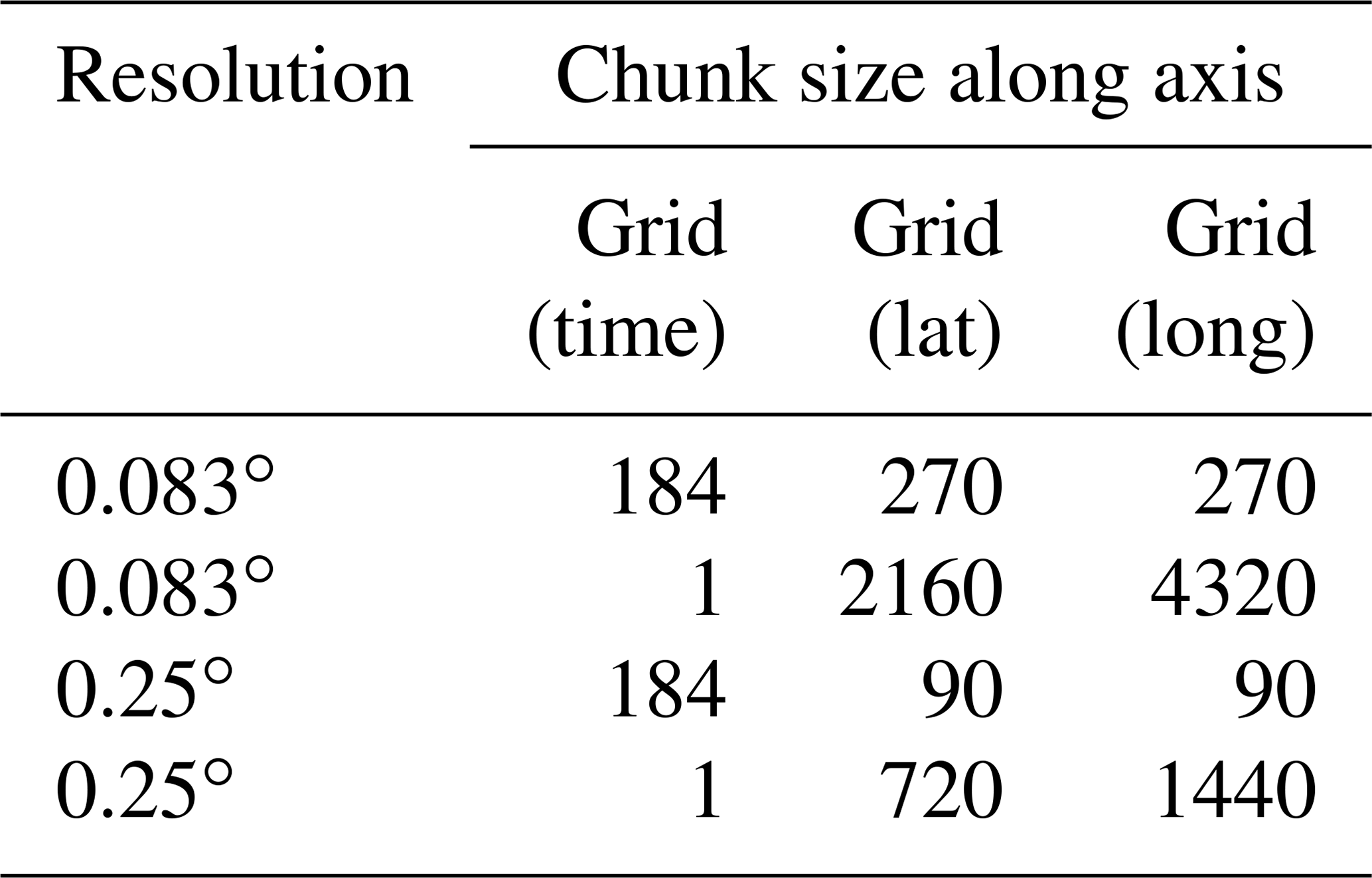
At present, the ESDL provides the same data cube in different spatial resolutions and different chunkings to speed up data access for different applications. In chunked data formats, a large data set is split into smaller chunks, which can be seen as separate entities where each chunk is represented by an object in an object store. There are several ways to chunk a data cube. Consider the case of a multivariate spatiotemporal cube 𝒞({lat, long, time, var}). One common strategy would be to treat every spatial map of each variable and time point as one chunk, which would result in a chunk size of |grid(lat)|×|grid(long). However, because an object can only be accessed as a whole, the time for reading a slice of a univariate data cube does not directly scale with the number of data points accessed but rather with the number of accessed chunks. Reading out a univariate time series of length 100 from this cube would require accessing 100 chunks. If one stored the same data cube with complete time series contained in one chunk, read operations could perform much faster. Table 2 shows an overview of the implemented chunkings for different cubes in the current ESDL environment.
Table 2Resolutions and chunkings of the currently implemented global Earth system data cube per variable. Here, the cubes with chunk size 1 in the time coordinate are optimized for accessing global maps at a time, while the other cubes are more suited for processing time series or regional subsets of the data cube. The cubes are currently hosted on the Object Storage Service by the Open Telecom Cloud under https://obs.eu-de.otc.t-systems.com/obs-esdc-v2.0.0/ (last access: 21 February 2020) (state: September 2019).
The overarching motivation for building an Earth system data cube is to support the multifaceted needs of Earth system sciences. Here, we briefly describe three case studies of varying complexity (estimating seasonal means per latitude, dimensionality reduction, and model–data integration) to illustrate how the concept of the Earth system data cube can be put into practice. Clearly, these examples emerge from our own research interest, but the concepts should be portable across different branches of science (the code for producing the results on display is provided as Jupyter notebooks at https://github.com/esa-esdl/ESDLPaperCode.jl, last access: 21 February 2020).
4.1 Inspecting summary statistics of biosphere–atmosphere interactions
Data exploration in the Earth system sciences typically starts with inspecting summary statistics. Global mean patterns across variables can give an impression on the long-term system behaviour across space. In this first use case, we aim to describe mean seasonal dynamics of multiple variables across latitudes.
Consider an input data cube of the form 𝒞({lat, long, time, var}). The first step consists in estimating the median seasonal cycles per grid cell. This operation creates a new dimension encoding the “day of year” (doy) as described in the atomic function of Eq. (9):
In a second step, we apply an averaging function that summarizes the dynamics observed at all longitudes:
The result is a cube of the form 𝒞({lat, doy, var}) describing the seasonal pattern of each variable per latitude. Figure 4 visualizes this analysis for data on GPP, air temperature (Tair), and surface moisture (SM; all references for data streams used are provided in Appendix A). The first row visualizes GPP; on the left side, we see the Northern Hemisphere, where darker colours describe higher latitudes and the background is the actual value of the variable. Together, the left and right plots describe the global dynamics of phenology, often referred to as the “green wave” (Schwartz, 1998). We clearly see the almost nonexistent GPP in high-latitude winters and also find the imprint of constantly low to intermediate productivity values at latitudes that are characterized by dry ecosystems. Pronounced differences between Northern and Southern Hemisphere reflect the very different distribution of productive land surface.
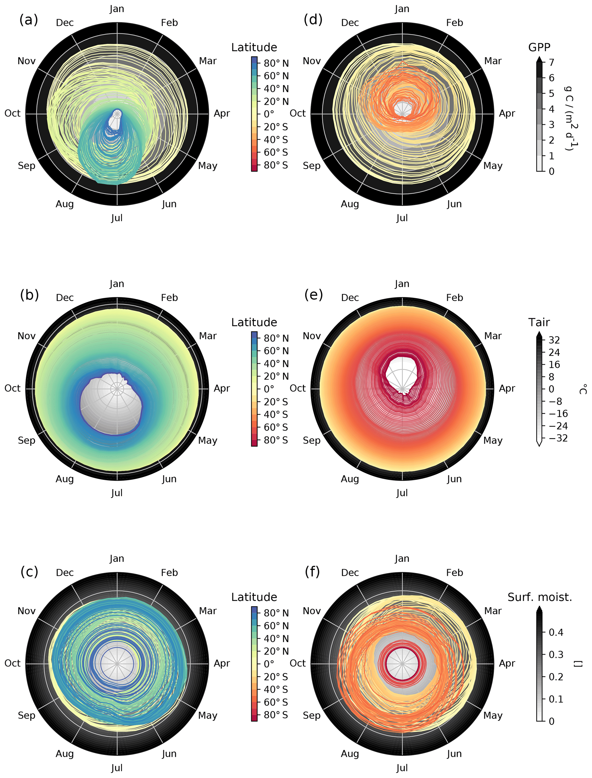
Figure 4Polar diagrams of median seasonal patterns per latitude (land only). The values of the variables are displayed as grey gradients and scale with the distance to the centroid. For each latitude, we have a median seasonal cycle specified with the central colour code. Panels (a–c) show the patterns for the Northern Hemisphere; panels (d–f) are the analogous figures for the Southern Hemisphere. Here, we show the patterns for GPP, air temperature at 2 m (Tair), and surface moisture (SM).
For temperature, the observed seasonal dynamics are less complex. We essentially find the constantly high temperature conditions near the Equator and visualize the pronounced seasonality at high latitudes. However, Fig. 4 also shows that temperature peaks lag behind the June/December solstices in the Northern Hemisphere, while in the Southern Hemisphere, the asymmetry of the seasonal cycle in temperature is less pronounced. While the seasonal temperature gradient is a continuum, surface moisture shows a much more complex pattern across latitudes, as reflected in summer/winter depressions in certain midlatitudes. For instance, a clear drop at, e.g. latitudes of approximately 60∘ N and even stronger depressions in latitudinal bands dominated by dry ecosystems.
This example analysis is intended to illustrate how the sequential application of two basic functions on this Earth system data cube can unravel global dynamics across multiple variables. We suspect that applications of this kind can lead to new insights into apparently known phenomena, as they allow to investigate a large number of data streams simultaneously and with consistent methodology.
4.2 Intrinsic dimensions of ecosystem dynamics
The main added value of the ESDL approach is its capacity to jointly analyse large numbers of data streams in integrated workflows. A long-standing question arising when a system is observed based on multiple variables is whether these are all necessary to represent the underlying dynamics. The question is whether the data observed in Y∈ℝM could be described with a vector space of much smaller dimensionality Z∈ℝm (where m≪M), without loss of information, and what value this “intrinsic dimensionality” m would have (Lee and Verleysen, 2007; Camastra and Staiano, 2016). Note that in this context the term “dimension” has a very different connotation compared to the “cube dimensions” introduced above.
When thinking about an Earth system data cube, the question about its intrinsic dimensionality could be investigated along the different axes. In this study, we ask if the multitude of data streams, grid(var), contained in our Earth system data cube is needed to grasp the complexity of the terrestrial surface dynamics. If the compiled data streams were highly redundant, it could be sufficient to concentrate on only a few orthogonal variables and design the development of the study accordingly. Starting from a cube 𝒞({lat, long, time, var}), we ask at each geographical coordinate if the local vector space spanned by the variables can be compressed such that mvar≪|grid(var)|.
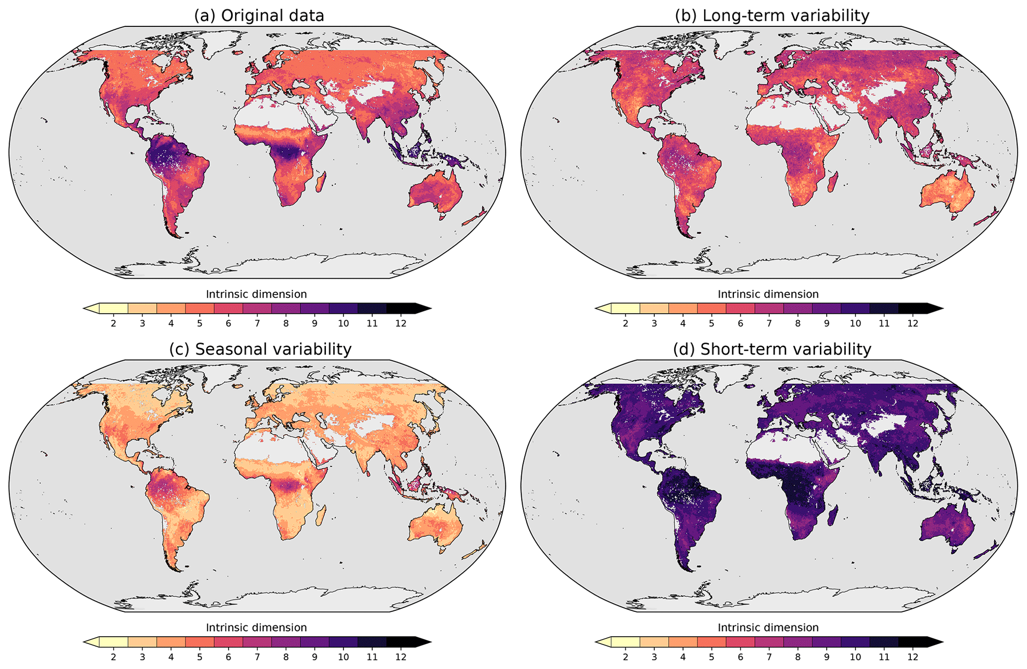
Figure 5Intrinsic dimension of 18 land ecosystem variables. The intrinsic dimension is estimated by counting how many principal components would be needed to explain at least 95 % of the variance in the Earth system data cube. The results for the original data are shown in panel (a). The analysis is then repeated based on subsignals of each variable, representing different timescales. In panel (b), we show the intrinsic dimension of long-term modes of variability, in (c) for modes representing seasonal components, and (d) for modes of short-term variability. Light grey areas indicate zones where at least one data stream was incomplete and no intrinsic dimension could be estimated based on the same set of variables.
Estimating the intrinsic dimension of high-dimensional data sets has been a matter of research for multiple decades, and we refer the reader to the existing reviews on the subject (e.g. Camastra and Staiano, 2016; Karbauskaite and Dzemyda, 2016). An intuitive approach is to measure the compressibility of a data set via dimensionality reduction techniques (see, e.g. van der Maaten et al., 2009; Kraemer et al., 2018). In the simplest case, one can apply a principal component analysis (PCA, using different time points as different observations) and estimate the number of components that together explain a predefined threshold of the data variance. In our application, we followed this approach and chose a threshold value of 95 % of variance. The atomic function needed for this study is described in Eq. (11):
The output is a map of spatially varying estimates of intrinsic dimensions mvar. We performed this study considering the following 18 variables relevant to describing land surface dynamics: GPP, Reco, NEE, LE, H, LAI, fAPAR, black- and white-sky albedo (each from two different sources), SMroot, S, transpiration, bare soil evaporation, evaporation, net radiation, and LST.
Figure 5 shows the results of this analysis for the original data, where the visualized range of intrinsic dimensions ranges from 2 to 13 (the analysis very rarely returns values of 1). At first glance, we find that ecosystems near the Equator are of higher intrinsic dimension (up to values of 12) compared to the rest of the land surface. In regions where we expect pronounced seasonal patterns, the intrinsic dimensionality is apparently low. We can describe these patterns by 4–7 dimensions. One explanation is that in cases where the seasonal cycle controls ecosystem dynamics, much of the surface variables tend to covary. This alignment implies that one can represent the dominant source of variance with few components of variability. In regions where the seasonal cycle plays only a marginal role, other sources of variability dominate that are, however, largely uncorrelated.
To verify that seasonality is the main source of variability in our analysis, we extend the workflow by decomposing each time series (by variable and spatial location) into a series of subsignals via a discrete fast Fourier transform (FFT). We then binned the subsignals into short-term, seasonal, and long-term modes of variability (as in Mahecha et al., 2010a; Linscheid et al., 2020), which leads to an extended data cube as we have shown in Eq. (12).
The resulting cube is then further processed in Eq. (13) (which is the analogue to Eq. 11) to extract the intrinsic dimension per timescale:
The timescale-specific intrinsic dimension estimates only partly confirm the initial conjecture (Fig. 5). Short-term modes of variability always show relatively high intrinsic dimensions; i.e. the high-frequency components in the variables are rather uncorrelated. This finding can either be a hint that we are seeing a set of independent processes or simply mean noise contamination. Seasonal modes, indeed, are of low intrinsic dimensionality, but considering that these modes are driven essentially by solar forcing only, they are surprisingly high dimensional. Additionally, we find a clear gradient from the inner tropics to arid and northernmost ecosystems. Warm and wet ecosystems seem to be characterized by a complex interplay of variables even when analysing their seasonal components only (see also Linscheid et al., 2020). One reason could be that seasonality in these regions is only marginally relevant to the total signal, or that tropical seasonality is inherently complicated. In the northern regions of South America, we find that arid regions seem to have low intrinsic seasonal dimensionality compared to more moist regions.
Long-term modes of land surface variability show a rather complex spatial pattern in terms of intrinsic dimensions: overall, we find values between 6 and 7 (see also the summary in Fig. 6). The values tend to be higher in high-altitude and tropical regions, whereas arid regions show low-complexity patterns. Long-term modes of variability in land surface variables are probably more complex than one would suspect a priori and should be analysed deeper in the near future.
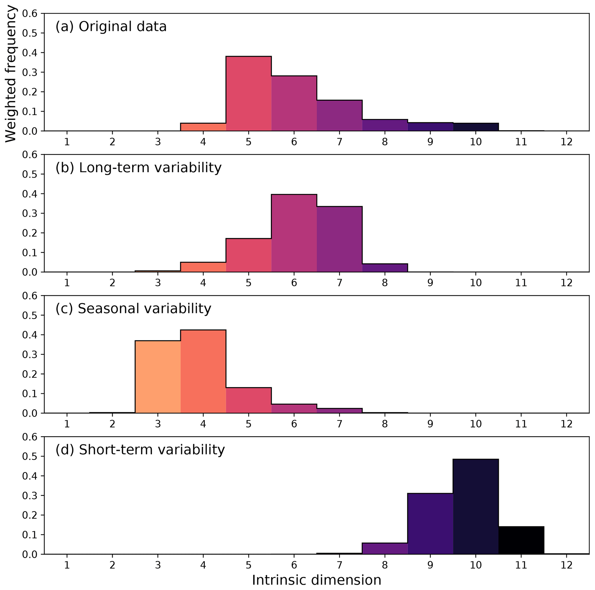
Figure 6Histogram of the intrinsic dimension estimated from 18 land ecosystem variables the Earth system data cube. The highest intrinsic dimension emerges in the short-term variability, while the original data are enveloped by the complexity of seasonal and long-term subsignals.
The analysis shows how a large number of variables can be seamlessly integrated into a rather complex workflow. However, the results should be interpreted with caution: one criticism of the PCA approach is its tendency to overestimate the correct intrinsic dimensions in the presence of nonlinear dependencies between variables. A second limitation is that the maximum intrinsic dimensions depend on the number of Fourier coefficients used to construct the signals, leading to different theoretical maximum intrinsic dimensions per timescale.
The question of the underlying dimensionality could also be investigated in a different way. While this study investigates the intrinsic dimensionality locally, i.e. along the dimensions of latitude and longitude, another recent study based on the ESDL by Kraemer et al. (2019) used a global PCA. Each observation is a point with coordinates “lat”, “long” and “time”, and the aim is to compress the “var” dimension. The form of the analysis is the following:
and was applied to a subset of ESDL variables that describe dynamics in terrestrial ecosystems. This study corroborates the idea that land surface dynamics can be well represented in a surprisingly low-dimensional space. The analysis presented by Kraemer et al. (2019) suggests globally a much lower intrinsic dimensionality of 3 compared to what we find here based on a grid-cell-level analysis. This number corresponds to areas that are marked by a strong seasonality in our case. This is plausible, because the areas that show high intrinsic dimensionality in Fig. 5 are those where seasonal variability is low compared to the high-frequency variability (Linscheid et al., 2020). Local effects of this kind vanish when all spatial points are jointly analysed.

Figure 7Global patterns of locally estimated temperature sensitivities of ecosystem respiration Q10 (a) via a conventional parameter estimation approach and (b) via a timescale-dependent parameter estimation method. The latter reduces the confounding influence of seasonality and leads to a fairly homogeneous map of temperature sensitivity.
4.3 Model parameter estimation in the ESDL
Another key element in supporting Earth system sciences with the ESDL (and related initiatives) is to enable model development, parameterization, and evaluation. To explore this potential, we present a parameter estimation study that considers two variables only, but it helps to illustrate the approach. In fact, the approach could be extended to exploit multiple data streams in complex models. The example presented here quantifies the sensitivities of ecosystem respiration – the natural release of CO2 by ecosystems – to fluctuations in temperature. Estimating such sensitivities is key for understanding and modelling the global climate–carbon cycle feedbacks (Kirschbaum, 1995). The following simple model (Davidson and Janssens, 2006) is widely used as a diagnostic description of this process:
where Reco,i is ecosystem respiration at time point i, and the parameter Q10 is the temperature sensitivity of this process, i.e. the factor by which Reco,i would change by increasing (or decreasing) the temperature Ti by 10 ∘C. An indication of how much respiration we would expect at some given reference temperature Tref is given by the pre-exponential factor Rb. Under this model, one can directly estimate the temperature sensitivities from some observed respiration and temperature time series. Technically, this is possible, and Eq. (16) describes a parameter estimation process as an atomic function:
that expects a multivariate time series and returns a parameter vector. Figure 7a visualizes these estimates, which are comparable to many other examples in the literature (see, e.g. Hashimoto et al., 2015) and depict pronounced spatial gradients. High-latitude ecosystems seem to be particularly sensitive to temperature variability according to such an analysis.
However, it has been shown theoretically (Davidson and Janssens, 2006), experimentally (Sampson et al., 2007), and using model–data fusion (Migliavacca et al., 2015), that the underlying assumption of a constant base rate is not justified. The reason is that the amount of respirable carbon in the ecosystem will certainly vary with the supply, and hence phenology, as well as with respiration-limiting factors such as water stress (Reichstein and Beer, 2008). In other words, ignoring the seasonal time evolution of Rb leads to substantially confounded parameter estimates for Q10.
One generic solution to the problem is to exploit the variability of respiratory processes at short-term modes of variability. Specifically, one can apply a timescale-dependent parameter estimation (SCAPE; Mahecha et al., 2010b), assuming that Rb varies slowly, e.g. on a seasonal and slower timescale. This approach requires some time series decomposition as described in Sect. 4.2. The SCAPE idea requires to rewrite the model, after linearization, such that it allows for a time-varying base rate:
The discrete spectral decomposition into frequency bands of the log-transformed respiration allows to estimate ln Q10 on specific timescales that are independent of phenological state changes (for an in-depth description, see Mahecha et al., 2010b, supporting materials). Conceptually, the model estimation process now involves two steps (Eqs. 18 and 19): a spectral decomposition where we produce a data cube of higher order,
followed by the parameter estimation, which differs from the approach described in Eq. (16), as this approach only returns a singular parameter (Q10), whereas ln Rb,i now becomes a time series:
The results of the analysis are shown in Fig. 7b, where we find generally a much more homogeneous and better constrained spatial pattern of Q10. As suggested in the site-level analysis by Mahecha et al. (2010b) and later by others (see, e.g. Wang et al., 2018), we find a global convergence of the temperature sensitivities. We also find that, e.g. semi-arid and savanna-dominated regions clearly show lower apparent Q10 (Fig. 7a) compared to the SCAPE approach (Fig. 7b). Discussing these patterns in detail is beyond the scope of this paper, but in general terms these findings are consistent with the expectation that in semi-arid ecosystems confounding factors act in the opposing direction (Reichstein and Beer, 2008).
Figure 8Bivariate histograms summarizing the joint distribution of surface moisture and gross primary production. The estimates are computed over the entire time series for the different Intergovernmental Panel on Climate Change (IPCC) regions. The density is square root transformed to emphasize areas of higher density. In arid regions (e.g. CAM, NEB, WAF, SAFM, EAF), the tight relation between surface water and primary production is evident.
From a more methodological point of view, this research application shows that it is well possible to implement a multistep analytic workflow in the ESDL that combines time series analysis and parameter estimation. Once the analysis is implemented, it requires essentially two sequential atomic functions. The results obtained have the form of a data cube and could be integrated into subsequent analyses. Examples include comparisons with in situ data, ecophysiological parameter interpretations, or assessment of parameter uncertainty in more detail. As mentioned above, this case study only considers two variables and thereby does not exploit the wider multivariate potential of the ESDL. The example of temperature sensitivity could easily be combined with further estimations of water stress, linked to primary production, or even become part of a simple terrestrial surface scheme.
4.4 Bivariate relations in vector cubes
The original idea of the data cube concept emerged from the need for working with large multivariate gridded data sets. However, the idea of data cubes can be possibly extended to other types of geographical data. One example is vector data cubes, where, e.g. polygons form an axis in their own right and each polygon points to a complex spatial shape. Consider, for instance, the need for statistical inferences on the spatial polygons often used in Intergovernmental Panel on Climate Change (IPCC) reports. One relevant question is, for example, understanding the relations of GPP and surface moisture. Figure 8 shows the bivariate histograms between both variables within a selected set of regions. This analysis clearly shows that in many regions of the world, GPP and surface moisture are strongly coupled. Examples are Central America/Mexico (CAM), north-east Brazil (NEB), west Africa (WAF), southern Africa (SAF), east Africa (EAF), south Asia (SAS), or south Australia/New Zealand (SAU). All of these regions contain significant fractions of semi-arid climates, which can explain the constraints that water availability has on photosynthetic CO2 uptake. In other regions, this relation is less obvious and often not pronounced, probably because the cases of water shortage are rare compared to the normal dynamics that might be constrained by other factors such as temperature. From a computational point of view, this example follows a very different logic, compared to the concept of applying an UDF on some of the cube axis. Rather, this example was computed using an “online” approach which sequentially updates some statistics (here the bivariate histograms) over a given class (here the IPCC regions). Such an approach allows calculations with large amounts of data and shows that the ESDL framework can also be coupled with conceptually very different analytical frameworks that might be particularly relevant when working with living data, i.e. with data streams that are constantly updated. In these cases, it is not desirable to constantly re-estimate all relevant quantities across the entire data cube.
In the following, we describe the insights gained during the development of the concept and the implementation of the ESDL, addressing issues arising and critiques expressed during our community consultation processes. We also briefly discuss the ESDL in light of other developments in the field. Finally, we highlight some challenges ahead and proposed future applications.
5.1 Insights and critical perspectives
During a community consultation process across various workshops and summer schools, users expressed confusion about the equitable treatment of data cube dimensions (Sect. 2). Considering that an unordered nominal dimension of “variables” is a dimension as “time” or “latitude” seems counterintuitive at first glance. Also, concerns have been expressed about whether “time” can be treated analogously to, e.g. “latitude”. Our main argument during the development of the ESDL was that it is possible, as long as the UDFs are not applied to dimensions where they would produce nonsense results. But the practical arguments for a common interface prevail. Also, and this is key, the concept and implementation are sufficiently flexible to allow users to deploy a more classical approach to deal with such data, e.g. analysing variables separately, or writing specific UDFs that specifically require spatial or temporal dimensions. However, for research examples structured like the second use case (Sect. 4.2), the proposed approach was key, as it is allowed to efficiently navigate through the variable dimension. It is obviously irrelevant to algorithms of dimensionality reduction which dimension is compressed, and we could have equally asked the question in time domain or across a spatial dimensions, which relates to the well-known empirical orthogonal functions (EOFs) as used in climate sciences (Storch and Zwiers, 1999). In exploratory approaches of this kind, where there is no prior scientific basis for presupposing where the “information-rich zones” are in the data cube, a dimension-agnostic approach clearly pays off. We also favour this idea as it is in-line with other approaches discussed in the community. For instance, the “data cube manifesto” (Baumann, 2017) states that “datacubes shall treat all axes alike, irrespective of an axis having a spatial, temporal, or other semantics”, a principle that we have radically implemented in the ESDL.jl Julia package (Sect. 3). The flexibility we gain is that we are, in principle, prepared for comparable cases where one has to deal with, e.g. multiple model versions, model ensemble members, or model runs based on varying initial conditions.
One of the most commonly expressed practical concerns is the choice of a unique data grid. The curation of multiple data streams within such a data cube grid requires that many data have to undergo reformatting and/or remapping. Of course, this can be problematic at times, in particular when data have been produced for a given spatial or temporal resolution and cannot be remapped without violating basic assumptions. For instance, keeping mass balances, integrals of flux densities, and global moments of intensive properties as consistent as possible should always be a priority. However, for the data cube approach implemented here, we decided to accept certain simplifications. The availability of a multitude of relevant data to study Earth system dynamics is a key incentive to use the ESDL and goes far beyond many disciplinary domains. But, as we have learned in this discussion, it comes at the price of some pragmatic trade-offs. A fundamental advancement of our approach would be to natively deal with data streams from unequal grids.
The current notation of the concept has been criticized for being unsuitable for dealing with so-called vector data cubes (Pebesma and Appel, 2019). Indeed, other conceptual approaches are more suited than ours to treat such examples (see, e.g. Gebbert et al., 2019). But the research example briefly described in Sect. 4.4 and Fig. 8 does showcase such a possibility. In this case, the idea of mapping a single function across some dimensions cannot be trivially realized, but it opens novel perspectives to compute statistics based on very big data. Further research needs to be done on developing the ESDL in such directions because it would allow not only for dealing with big data issues but also to update statistics without having to recompute data processed in earlier steps. This can solve the challenges of dealing with “living data”.
One of the main concerns expressed by users, in particular by 30 young researchers who participated in the project during an early adopter phase, is the demand for the latest data in the ESDL. This is why the concept presented here and its implementation should be further developed into a persistent infrastructure. Such a step is challenging and there is a trade-off to be made between wishing to include latest data streams (ideally even in near-real time) and constantly expanding the access API and portfolio of example workflows. The ESDL thus depends on the enduring enthusiasm of the user community and funding agencies to support the idea in this respect and grow steadily into new domains, help us add data streams, and actively co-develop the approach.
5.2 Relation to other initiatives and platforms
Over the past few years, several initiatives, platforms, and software solutions (Lu et al., 2018; Sudmanns et al., 2019) have emerged based on similar considerations as those motivating the Earth System Data Lab. Some of these platforms and software solutions are explicitly constructed around the idea of data cubes (e.g. Baumann et al., 2016; Lewis et al., 2017; Appel and Pebesma, 2019). Nevertheless, the concept of “data cube” is still not fully consolidated in the Earth system science. It was only in 2019 that the Open Geospatial Consortium (OGC) opened a public discussion towards establishing standards for data cubes.
Among the other existing initiatives, the Climate Data Store (CDS) of the Copernicus Climate Change Service (https://cds.climate.copernicus.eu/, last access: 21 February 2020) is conceptually probably the closest one to the ESDL. The CDS was primarily designed as key infrastructure to analyse climate reanalysis data and related variables. These data often require to be analysed at very high temporal resolutions (e.g. using hourly time steps). The CDS offers a similar Python interface to analyse these data. Likewise, the Google Earth Engine (GEE; https://earthengine.google.com, last access: 21 February 2020; Gorelick et al., 2017) is probably the most widely known platform for implementing global-scale analytics. GEE offers access to a wide range of satellite data archives and increasingly also to climate data in their native resolutions. One strength of GEE is the massive computing power offered to the scientist, such that some use cases nicely showcased the power of the infrastructure. The user has a wide range of predefined operators available that can be used and coupled to build workflows that are particularly suitable for time series. Another recent development in the field is the Open Data Cube (ODC; https://www.opendatacube.org/, last access: 21 February 2020; formerly Australian Data Cube; Lewis et al., 2017). This project was initially designed to offer access to the well-processed remote sensing data over Australia with an emphasis on the Landsat archive. In the past years, the ODC technology was used to implement regional data cubes for Colombia (CDCol; Ariza-Porras et al., 2017; Bravo et al., 2017), Switzerland (SDC; http://www.swissdatacube.org/, last access: 21 February 2020; Giuliani et al., 2017), and Armenia (Asmaryan et al., 2019), among many other countries. The aim of the open-access ODC is also to effectively enable access to time series data from high-resolution data archives, targeting mainly changes in land surface properties. The ESDL has developed into a conceptually different direction than most of the other initiatives that make it unique.
First, we note that most of the data cube initiatives were motivated by the need to access and/or analyse big, e.g. very-high-resolution, data (Lewis et al., 2017; Nativi et al., 2017; Giuliani et al., 2019). Initially, this problem was not in the focus of the ESDL, which rather aimed at downstream data products. Our data cube approach primarily intends to support the joint exploitation of multiple data streams efficiently. This multivariate focus is rarely found as a key design element in the other approaches.
Second, most initiatives intend to preserve the resolutions of the underlying data. The ESDL, instead, is built around singular data cubes that then include variables as an additional dimension. The inevitable trade-off, as discussed above, is the need for a data curation and remapping process prior to the analyses.
Third, there is a wide consensus that data cube technologies need to enable the application of UDFs. However, at this stage, this aspect often appears not to be a priority of other data cube initiatives and, consequently, users are restricted in their analysis by the available tools. In this context, we see the strength of the ESDL, as it allows for the development of complex workflows and adding arbitrary functionalities efficiently. This is actually one reason why we decided to implement the ESDL in the quite young language of scientific computing Julia (side by side with the more commonly used Python tools).
Taken together, the ESDL has probably conceptually developed (and implemented) the most radical cubing principle following a strict dimension agnostic approach. We envisage that the ESDL front end could be coupled to a data cube technology as proposed by any of the other initiatives to combine its analytic strength with the efficiencies achieved by others in dealing with high-resolution data streams.
5.3 Priorities for future developments
During the development of the ESDL, we identified several methodological challenges on the one hand and, on the other, application domains that could be addressed. With regard to potentially relevant methodological paths, we can only briefly mention, with no claim to completeness, some of the most ardently and widely discussed topics:
-
Machine learning. Data-driven approaches have always been part of the DNA of Earth system sciences (see classical textbooks, e.g. Storch and Zwiers, 1999) and classically complement process-driven modelling efforts (Luo et al., 2012). However, with the rise of modern machine learning, new perspectives have emerged (Mjolsness and DeCoste, 2001; Hsieh, 2009). Depending on the purpose, we find purely exploratory analysis based on, e.g. nonlinear dimensionality reduction (Mahecha et al., 2010a) or predictive techniques (Jung et al., 2009) being transferred from computer sciences to the Earth system sciences. Today, deep learning is on everybody's lips and could mark one step forward in Earth system science (Karpatne et al., 2018; Shen et al., 2018; Bergen et al., 2019; Reichstein et al., 2019). Through providing an easy access to relevant data streams, the Earth system data cube idea may attract further researchers from data sciences into the field. It furthermore provides the perfect platform for studying complex tasks such as detecting multidimensional extreme events (Flach et al., 2017), characterization of information content and dependencies in the data with information-theoretic measures (Sippel et al., 2016), or causal inference (Runge et al., 2019; Pearl, 2009; Peters et al., 2017; Christiansen and Peters, 2020; Krich et al., 2019). We believe that the clear and easy-to-use interface of the ESDL renders it well suited for being part of machine learning challenges such as the ones organized by Kaggle (https://www.kaggle.com/competitions, last access: 21 February 2020) or during premier conferences of the field.
-
Spatial interactions. For interpreting the interactions and mechanisms of the land and ocean, or land and atmosphere that involve lateral transport, the ESDL would require more developments. Statistical approaches like spatial network analyses (e.g. Donges et al., 2009; Boers et al., 2019) or process-oriented ideas like explicit moisture transport (e.g. Wang-Erlandsson et al., 2018) would be very valuable to be explored but would require a substantial rethinking of the actual implementation in order to achieve high performance.
-
Model evaluation and benchmarking. Our third use case (Sect. 4.3) illustrates the suitability of the ESDL for parameter estimation and model evaluation purposes. Today, typical model evaluation frameworks in the Earth system sciences prepare predefined benchmark metrics on some reference data sets (Luo et al., 2012). Prominent examples are the benchmarking tools awaiting the sixth phase of the Coupled Model Intercomparison Project (CMIP6) model suites (Eyring et al., 2019). However, these model evaluation frameworks typically do not give the user the full flexibility to apply some user-defined metrics to the model ensemble under scrutiny. We believe that mapping UDFs on such big Earth system model output could greatly benefit the development of novel evaluation metrics in the near future. Building data cubes from multi-model ensembles would be straightforward, as different models or ensembles would simply lead to one additional dimension in our setup. In fact, the ESDL approach is perfectly suited to handle, e.g. the output of the actual CMIP data, as we have already exemplified2. Of course, any other model ensembles can be treated analogously.
In terms of application domains, we see high potential in the following areas:
-
Human–environment interactions. Addressing the complexities of human–environment interactions (Schimel et al., 2015) is a particular challenge. Making the ESDL fit for this purpose would require integrating a variety of (at least) spatially explicit population estimates (Doxsey-Whitfield et al., 2015) and socioeconomic data Smits and Permanyer (2019). The latter represent a fundamentally novel development that has great potential for understanding, e.g. dynamics of disaster impacts (Guha-Sapir and Checchi, 2018), among other issues. In fact, this integration is a grand challenge ahead (Mahecha et al., 2019) but not out of reach for the ESDL.
-
Biodiversity research. Another question of high societal relevance is to understand how patterns of biodiversity affect ecosystem functioning (Emmett Duffy et al., 2017; García-Palacios et al., 2018). In light of a global decline in species richness (see latest global reports; https://www.ipbes.net/, last access: 21 February 2020), this question is of uttermost importance. The ESDL is only partly fit for this purpose, as it would require the ingestion of a wide range of essential biodiversity variables (Pereira et al., 2013; Skidmore et al., 2015), beyond the ones we have already available. But still, the ESDL is conceptually prepared to deal with these challenges (compare, e.g. the demands described in Hardisty et al., 2019) and would be particularly suitable for relating biodiversity patters to the so-called ecosystem function properties (Reichstein et al., 2014; Musavi et al., 2015). In fact, in the regional application of the ESDL, we have focused on Colombia and its wider region to explore linkages of this kind relying on remote-sensing-derived variables that are relevant for this context.
-
Oceanic sciences. Extending the ESDL for ocean data is desired and conceptually possible. Surface parameters, e.g. phytoplankton phenology derived from remote sensing (Racault et al., 2012), can be treated analogously to terrestrial surface parameters. Other dynamics, e.g. the analysis and exploration of ocean–land coupling mechanisms, ocean–atmosphere interactions, and land–atmosphere interactions triggered by ocean circulation dynamics, could in principle be facilitated via the ESDL but require either vertical or lateral dynamics.
-
Solid Earth. The step towards global, fully data informed model data is also made in geophysics. For instance, recently Afonso et al. (2019) used an inversion approach to develop a 3-D model that fully describes multiple parameters in the Earth interior, including, e.g. crustal and lithospheric thickness, average crustal density, and a depth-dependent density of the lithospheric mantle, among other variables. They proposed a tool allowing for inspecting the data interactively at a spatial resolution of 2∘ × 2∘ grid at different depths. Clearly, in this case, other dimensions are relevant, but the principle remains the same and, in fact, can be treated in a very similar manner. Future model–data assimilation approaches of this kind could be performed in the context of the ESDL, as well as the aforementioned machine learning for the solid Earth (Bergen et al., 2019).
In summary, we have demonstrated that the ESDL is a flexible and generic framework that can allow various different communities to explore and analyse large amounts of gridded data efficiently. Thinking about the potential paths ahead, the ESDL could become a valuable tool in various fields of Earth system sciences, biodiversity research, computer sciences, and other branches of science. The widespread social and political uptake of the concept of planetary boundaries (Rockström et al., 2009; Steffen et al., 2015) underlines the global demand for better quantified process understanding of environmental risks and resource bottlenecks based on empirical evidence. Along these lines, the ESDL concept could be used to address some of the most pressing global challenges. For example, it could become an interface for direct interaction with ECVs, global climate projections, and EBVs. Such an interactive interface would allow a much broader community to better understand the data underlying the global assessment reports of the IPCC (IPCC, 2014) and Intergovernmental Science-Policy Platform on Biodiversity and Ecosystem Services (IPBES) (Diaz et al., 2019). If coupled to some visual interfaces, the ESDL could also be used by a broader community, enhancing education, communication, and decision-making process, contributing to knowledge democratization about a deeper understanding of the complex and dynamic interactions in the Earth system.
Exploiting the synergistic potential of multiple data streams in the Earth sciences beyond disciplinary boundaries requires a common framework to treat multiple data dimensions, such as spatial, temporal, variable, frequency, and other grids alike. This idea leads to a data cube concept that opens novel avenues to efficiently deal with data in the Earth system sciences. In this paper, we have formalized the concept of data cubes and described a way to operate on them. The outlined dimension-agnostic approach is implemented in the Earth System Data Lab, which enables users applying a wide range of functions to all thinkable combinations of dimension. We believe that this idea can dramatically reduce the barrier to exploit Earth system data and serves multiple research purposes. The ESDL complements a range of emerging initiatives that differ in architectures and specific purposes. However, the ESDL is probably the most radical data cubing approach, offering novel opportunities for cross-community data-intensive exploration of contemporary global environmental changes. Future developments in related branches of science and latest methodological developments need to be considered and addressed soon. At its actual state of implementation, the ESDL can already contribute to the deeper understanding and more effective implementation of policy-relevant concepts such as the planetary boundaries, essential variables in different subsystems of the Earth, and global assessment reports. We see a particularly high future potential for data cube concepts as presented for, firstly, interpreting large-scale model ensembles, and secondly, analysing new multispectral satellite remote sensing data with their constantly increasing spatial, temporal, and spectral resolutions.
In the following, we give an overview of the actually available variables in the Earth System Data Lab. The list is constantly being updated.
Dee et al. (2011)Holzer-Popp et al. (2013)Holzer-Popp et al. (2013)Holzer-Popp et al. (2013)Holzer-Popp et al. (2013)Holzer-Popp et al. (2013)Tramontana et al. (2016)Tramontana et al. (2016)Tramontana et al. (2016)Tramontana et al. (2016)Giglio et al. (2013)Giglio et al. (2013)van der Werf et al. (2017)Martens et al. (2017)Miralles et al. (2011)Martens et al. (2017)Miralles et al. (2011)Martens et al. (2017)Miralles et al. (2011)Martens et al. (2017)Miralles et al. (2011)Martens et al. (2017)Miralles et al. (2011)Martens et al. (2017)Miralles et al. (2011)Martens et al. (2017)Miralles et al. (2011)Martens et al. (2017)Miralles et al. (2011)Martens et al. (2017)Miralles et al. (2011)Martens et al. (2017)Miralles et al. (2011)Lewis et al. (2012)Lewis et al. (2012)Luojus et al. (2010)Metsämäki et al. (2015)Luojus et al. (2010)Ghent (2012)Schröder et al. (2012)Schneider et al. (2013)Adler et al. (2003)Huffman et al. (2009)Van Roozendael et al. (2012)Lerot et al. (2014)Pinty et al. (2006)Disney et al. (2016)Blessing and Löw (2017)Pinty et al. (2006)Disney et al. (2016)Blessing and Löw (2017)Lewis et al. (2012)Danne et al. (2017)Lewis et al. (2012)Danne et al. (2017)Gobron et al. (2017)Liu et al. (2012)Dorigo et al. (2017)Gruber et al. (2017)
All code necessary to build and analyse the ESDL is available from https://github.com/esa-esdl (last access: 21 February 2020) (Fomferra, 2020). The case studies presented in Sect. 4 can be fully reproduced from https://github.com/esa-esdl/ESDLPaperCode.jl (last access: 21 February 2020), https://doi.org/10.5281/zenodo.3670743 (Gans, 2020).
All data are available via https://www.earthsystemdatalab.net/ (last access: 21 February 2020) or from the original data providers as indicated in Table A1 in the paper.
MDM, FG, and MR developed the concept; FG implemented
the ESDL.jl package in the Julia language; NF, FG, MDM,
and GB implemented the overall project; MCL and LES implemented the Colombian cube. RC, JP, MDM, FG, GK, PB, and PP developed the notation; DGM and MJ contributed particular data. MDM wrote the manuscript with substantial input from FG, SC, GCV, RC, JP, and GK, and detailed comments from all co-authors.
The authors declare that they have no conflict of interest.
This paper was funded by the European Space Agency (ESA) via the Earth System Data Lab (ESDL) project. The authors also thank the Integrated Land Ecosystem Atmosphere Processes Study (iLEAPS), a FutureEarth Global Research Project for constant support. Special thanks are given to Anca Anghelea, Eleanor Blyth, Carsten Brockmann, Diego Fernández, Garry Hayman, Toby R. Marthews, Pierre-Philippe Mathieu, Espen Volden, and Uli Weber for continuous support and feedback. We also thank everyone participating in the various workshops and summer schools, and especially the young scientists participating in the “early adopters” call, for providing invaluable feedback on the development of the ESDL. Marius Appel, Edzer Pebesma, Alexander Winkler, and two anonymous referees provided excellent comments on the manuscript. The implementation of the regional Earth data cube for Colombia was done under the project “Champion user phase; Supporting the Colombia BON in GEO BON” with the ESDL project. The original idea emerged at the iLEAPS–ESA–MPG-funded workshop in Frascati 2011 (Mahecha et al., 2011). We thank everyone who made data freely available such that they could be used in this project. Rune Christiansen and Jonas Peters were supported by a research grant (18968) from VILLUM FONDEN. Gustau Camps-Valls was supported by the ERC under ERC-COG-2014 SEDAL (grant agreement no. 647423); Diego G. Miralles was supported by the ERC under grant agreement no. 715254 (DRY-2-DRY). Jonathan F. Donges was supported by the Stordalen Foundation (via the Planetary Boundary Research Network) and the ERC via the ERC advanced grant project ERA (Earth resilience in the Anthropocene). Lina M. Estupinan-Suarez was supported by the DAAD programme 57315018.
This research has been supported by the European Space Agency (project Earth System Data Lab).
The article processing charges for this open-access
publication were covered by the Max Planck Society.
This paper was edited by Kirsten Thonicke and reviewed by two anonymous referees.
Adler, R. F., Huffman, G. J., Chang, A., Ferraro, R., Xie, P.-P., Janowiak, J., Rudolf, B., Schneider, U., Curtis, S., Bolvin, D., Gruber, A., Susskind, J., Arkin, P., and Nelkin, E.: The Version-2 Global Precipitation Climatology Project (GPCP) Monthly Precipitation Analysis (1979–Present), J. Hydrometeorol., 4, 1147–1167, https://doi.org/10.1175/1525-7541(2003)004<1147:TVGPCP>2.0.CO;2, 2003. a, b
Afonso, J. C., Salajegheh, F., Szwillus, W., Ebbing, J., and Gaina, C.: A global reference model of the lithosphere and upper mantle from joint inversion and analysis of multiple data sets, Geophys. J. Int., 217, 1602–1628, https://doi.org/10.1093/gji/ggz094, 2019. a
Appel, M. and Pebesma, E.: On-Demand Processing of Data Cubes from Satellite Image Collections with the gdalcubes Library, Data, 4, 92, https://doi.org/10.3390/data4030092, 2019. a, b
Ariza-Porras, C., Bravo, G., Villamizar, M., Moreno, A., Castro, H., Galindo, G., Cabera, E., Valbuena, S., and Lozano, P.: CDCol: A geoscience data cube that meets colombian needs, in: Advances in Computing, CCC 2017, Communications in Computer and Information Science, vol. 735, edited by: Solano, A. and Ordoñez, H., Springer, Cham, 87–99, 2017. a
Asmaryan, S., Muradyan, V., Tepanosyan, G., Hovsepyan, A., Saghatelyan, A., Astsatryan, H., Grigoryan, H., Abrahamyan, R., Guigoz, Y., and Giuliani, G.: Paving the way towards an armenian data cube, Data, 4, 117, 2019. a
Baldocchi, D.: Measuring fluxes of trace gases and energy between ecosystems and the atmosphere – the state and future of the eddy covariance method, Global Change Biol., 20, 3600–3609, https://doi.org/10.1111/gcb.12649, 2014. a
Balsamo, G., Agusti-Panareda, A., Albergel, C., Arduini, G., Beljaars, A., Bidlot, J., Bousserez, N., Boussetta, S., Brown, A., Buizza, R., Buontempo, C., Chevallier, F., Choulga, M., Cloke, H., Cronin, M. F., Dahoui, M., Rosnay, P. D., Dirmeyer, P. A., Drusch, M., Dutra, E., Ek, M. B., Gentine, P., Hewitt, H., Keeley, S. P., Kerr, Y., Kumar, S., Lupu, C., Mahfouf, J.-F., McNorton, J., Mecklenburg, S., Mogensen, K., Muñoz-Sabater, J., Orth, R., Rabier, F., Reichle, R., Ruston, B., Pappenberger, F., Sandu, I., Seneviratne, S. I., Tietsche, S., Trigo, I. F., Uijlenhoet, R., Wedi, N., Woolway, R. I., and Zeng, X. : Satellite and in situ observations for advancing global Earth surface modelling: A Review, Remote Sensing, 10, 2038, https://doi.org/10.3390/rs10122038, 2018. a
Baumann, P.: The datacube manifesto, available at: https://external.opengeospatial.org/twiki_public/pub/CoveragesDWG/Datacubes/The-Datacube-Manifesto.pdf (last access: 24 February 2020), 2017. a
Baumann, P., Dehmel, A., Furtado, P., Ritsch, R., and Widmann, N.: The Multidimensional Database System RasDaMan, in: Proceedings of the 1998 ACM SIGMOD International Conference on Management of Data, SIGMOD '98, ACM, New York, NY, USA, 575–577, https://doi.org/10.1145/276304.276386, 1998. a
Baumann, P., Mazzetti, P., Ungar, J., Barbera, R., Barboni, D., Beccati, A., Bigagli, L., Boldrini, E., Bruno, R., Calanducci, A., Campalani, P., Clements, O., Dumitru, A., Grant, M., Herzig, P., Kakaletris, G., Laxton, J., Koltsida, P., Lipskoch, K., Mahdiraji, A. R., Mantovani, S., Merticariu, V., Messina, A., Misev, D., Natali, S., Nativi, S., Oosthoek, J., Pappalardo, M., Passmore, J., Rossi, A. P., Rundo, F., Sen, M., Sorbera, V., Sullivan, D., Torrisi, M., Trovato, L., Veratelli, M. G., and Wagner, S.: Big Data Analytics for Earth Sciences: the EarthServer approach, Int. J. Digit. Earth, 9, 3–29, https://doi.org/10.1080/17538947.2014.1003106, 2016. a, b, c
Bergen, K. J., Johnson, P. A., Maarten, V., and Beroza, G. C.: Machine learning for data-driven discovery in solid Earth geoscience, Science, 363, eaau0323, https://doi.org/10.1126/science.aau0323, 2019. a, b, c
Bezanson, J., Edelman, A., Karpinski, S., and Shah, V.: Julia: A Fresh Approach to Numerical Computing, SIAM Rev., 59, 65–98, https://doi.org/10.1137/141000671, 2017. a
Blessing, S. and Löw, A.: Product User Guide for QA4ECV-TIP-BHR-LAI/FAPAR, available at: http://www.qa4ecv-land.eu/docs/D4.6-PUG_all_20170210.pdf (last access: 22 February 2020), 2017. a, b, c
Bodesheim, P., Jung, M., Gans, F., Mahecha, M. D., and Reichstein, M.: Upscaled diurnal cycles of land–atmosphere fluxes: a new global half-hourly data product, Earth Syst. Sci. Data, 10, 1327–1365, https://doi.org/10.5194/essd-10-1327-2018, 2018. a
Boers, N., Goswami, B., Rheinwalt, A., Bookhagen, B., Hoskins, B., and Kurths, J.: Complex networks reveal global pattern of extreme-rainfall teleconnections, Nature, 566, 373–377, https://doi.org/10.1038/s41586-018-0872-x, 2019. a
Bojinski, S., Verstraete, M., Peterson, T. C., Richter, C., Simmons, A., and Zemp, M.: The concept of essential climate variables in support of climate research applications, and policy, B. Am. Meteorol. Soc., 95, 1431–1443, https://doi.org/10.1175/BAMS-D-13-00047.1, 2014. a
Bravo, G., Castro, H., Moreno, A., Ariza-Porras, C., Galindo, G., Cabrera, E., Valbuena, S., and Lozano-Rivera, P.: Architecture for a Colombian data cube using satellite imagery for environmental applications, in: Colombian Conference on Computing, Springer, 227–241, available at: https://www.springerprofessional.de/en/architecture-for-a-colombian-data-cube-using-satellite-imagery-f/14221178 (last access: 22 February 2020), 2017. a
Camastra, F. and Staiano, A.: Intrinsic dimension estimation: Advances and open problems, Inform. Sci., 328, 26–41, https://doi.org/10.1016/j.ins.2015.08.029, 2016. a, b
Camps-Valls, G., Sejdinovic, D., Runge, J., and Reichstein, M.: A Perspective on Gaussian Processes for Earth Observation, Nat. Sci. Rev., 6, 616–618, https://doi.org/10.1093/nsr/nwz028, 2019. a
Christiansen, R. and Peters, J.: Switching regression models and causal inference in the presence of discrete latent variables, J. Mach. Learn. Res., in press, 2020. a
Danne, O., Muller, J. P., Kharbouche, S., and Lattanzio, A.: Product User Guide for QA4ECV-albedo, available at: http://www.qa4ecv-land.eu/docs/D4.6-PUG_all_20170210.pdf (last access: 22 February 2020), 2017. a, b
Davidson, E. A. and Janssens, I. A.: Temperature sensitivity of soil carbon decomposition and feedbacks to climate change, Nature, 440, 165–173, https://doi.org/10.1038/nature04514, 2006. a, b
Dee, D. P., Uppala, S. M., Simmons, A. J., Berrisford, P., Poli, P., Kobayashi, S., Andrae, U., Balmaseda, M. A., Balsamo, G., Bauer, P., Bechtold, P., Beljaars, A. C. M., van de Berg, L., Bidlot, J., Bormann, N., Delsol, C., Dragani, R., Fuentes, M., Geer, A. J., Haimberger, L., Healy, S. B., Hersbach, H., Hólm, E. V., Isaksen, L., Kållberg, P., Köhler, M., Matricardi, M., McNally, A. P., Monge-Sanz, B. M., Morcrette, J.-J., Park, B.-K., Peubey, C., de Rosnay, P., Tavolato, C., Thépaut, J.-N., and Vitart, F.: The ERA-Interim reanalysis: configuration and performance of the data assimilation system, Q. J. Roy. Meteorol. Soc., 137, 553–597, https://doi.org/10.1002/qj.828, 2011. a
Diaz, S., Settele, J., Brondízio, E., Ngo, H., Guèze, M., Agard, J., Arneth, A., Balvanera, P., Brauman, K., Butchart, S., Chan, K., Garibaldi, L. A., Ichii, K., Liu, J., Subramanian, S. M., Midgley, G. F., Miloslavich, P., Molnár, Z., Obura, D., Pfaff, A., Polasky, S., Purvis, A., Razzaque, J., Reyers, B., Chowdhury, R. R., Shin, Y.-J., Visseren-Hamakers, I., Willis, K., and Zayas, C.: Summary for policymakers of the global assessment report on biodiversity and ecosystem services of the Intergovernmental Science-Policy Platform on Biodiversity and Ecosystem Services, available at: https://ipbes.net/global-assessment (last access: 22 February 2020), 2019. a
Disney, M., Muller, J.-P., Kharbouche, S., Kaminski, T., Voßbeck, M., Lewis, P., and Pinty, B.: A New Global fAPAR and LAI Dataset Derived from Optimal Albedo Estimates: Comparison with MODIS Products, Remote Sensing, 8, 275, https://doi.org/10.3390/rs8040275, 2016. a, b, c
Donges, J. F., Zou, Y., Marwan, N., and Kurths, J.: Complex networks in climate dynamics. Comparing linear and nonlinear network construction methods, Eur. Phys. J.-Spec. Top., 174, 157–179, https://doi.org/10.1140/epjst/e2009-01098-2, 2009. a
Dorigo, W., Wagner, W., Albergel, C., Albrecht, F., Balsamo, G., Brocca, L., Chung, D., Ertl, M., Forkel, M., Gruber, A., Haas, E., Hamer, P. D., Hirschi, M., Ikonen, J., de Jeu, R., Kidd, R., Lahoz, W., Liu, Y. Y., Miralles, D., Mistelbauer, T., Nicolai-Shaw, N., Parinussa, R., Pratola, C., Reimer, C., van der Schalie, R., Seneviratne, S. I., Smolander, T., and Lecomte, P.: ESA CCI Soil Moisture for improved Earth system understanding: State-of-the art and future directions, Remote Sens. Environ., 203, 185–215, https://doi.org/10.1016/j.rse.2017.07.001, 2017. a
Dorigo, W. A., Wagner, W., Hohensinn, R., Hahn, S., Paulik, C., Xaver, A., Gruber, A., Drusch, M., Mecklenburg, S., van Oevelen, P., Robock, A., and Jackson, T.: The International Soil Moisture Network: a data hosting facility for global in situ soil moisture measurements, Hydrol. Earth Syst. Sci., 15, 1675–1698, https://doi.org/10.5194/hess-15-1675-2011, 2011. a
Doxsey-Whitfield, E., MacManus, K., Adamo, S. B., Pistolesi, L., Squires, J., Borkovska, O., and Baptista, S. R.: Taking advantage of the improved availability of census data: a first look at the gridded population of the world, version 4, Pap. Appl. Geogr., 1, 226–234, 2015. a
Duveiller, G. and Cescatti, A.: Spatially downscaling sun-induced chlorophyll fluorescence leads to an improved temporal correlation with gross primary productivity, Remote Sens. Environ., 182, 72–89, https://doi.org/10.1016/j.rse.2016.04.027, 2016. a
Emmett Duffy, J., Godwin, C., and Cardinale, B.: Biodiversity effects in the wild are common and as strong as key drivers of productivity, Nature, 549, 261–264, https://doi.org/10.1038/nature23886, 2017. a
Eyring, V., Cox, P., Flato, G., Gleckler, P., Abramowitz, G., Caldwell, P., Collins, W., Gier, B., Hall, A., Hoffman, F., Hurtt, G., Jahn, A., Jones, C., Klein, S., Krasting, J., Kwiatkowski, L., Lorenz, R., Maloney, E., Meehl, G., Pendergrass, A., Pincus, R., Ruane, A., Russell, J., Sanderson, B., Santer, B., Sherwood, S., Simpson, I., Stouffer, R., and Williamson, M.: Taking climate model evaluation to the next level, Nat. Clim. Change, 9, 102–110, https://doi.org/10.1038/s41558-018-0355-y, 2019. a, b
Flach, M., Gans, F., Brenning, A., Denzler, J., Reichstein, M., Rodner, E., Bathiany, S., Bodesheim, P., Guanche, Y., Sippel, S., and Mahecha, M. D.: Multivariate anomaly detection for Earth observations: a comparison of algorithms and feature extraction techniques, Earth Syst. Dynam., 8, 677–696, https://doi.org/10.5194/esd-8-677-2017, 2017. a
Flórez, C., Estupiñán-Suárez, L., Rojas, S., Aponte, C., Quiñones, M., Acevedo, O., Vilardy, S., and Jaramillo, U.: Identificación espacial de los sistemas de humedales continentales de Colombia, Biota Colombiana, 17, 44–62, https://doi.org/10.21068/c2016s01a03, 2016. a
Fomferra, N.: ESA Earth System Laboratory, available at: https://github.com/esa-esdl, last access: 21 February 2020). a
Gans, F.: Final version of the Data cube paper code, https://doi.org/10.5281/zenodo.3670743, 2020. a
García-Palacios, P., Gross, N., Gaitán, J., and Maestre, F. T.: Climate mediates the biodiversity–ecosystem stability relationship globally, P. Natl. Acad. Sci. USA, 115, 8400–8405, https://doi.org/10.1073/pnas.1800425115, 2018. a
Gebbert, S., Leppelt, T., and Pebesma, E.: A topology based spatio-temporal map algebra for big data analysis, Data, 4, 86, https://doi.org/10.3390/data4020086, 2019. a
Ghent, D.: Land Surface Temperature Validation and Algorithm Verification. Report to European Space Agency, available at: https://earth.esa.int/documents/700255/2411932/QC3_D4.1+Validation_Report_Issue_1A_20120416.pdf (last access: 22 February 2020), 2012. a
Giglio, L., Randerson, J. T., and Werf, G. R.: Analysis of daily, monthly, and annual burned area using the fourth-generation global fire emissions database (GFED4), J. Geophys. Res.-Biogeo., 118, 317–328, https://doi.org/10.1002/jgrg.20042, 2013. a, b
Giuliani, G., Chatenoux, B., De Bono, A., Rodila, D., Richard, J.-P., Allenbach, K., Dao, H., and Peduzzi, P.: Building an earth observations data cube: lessons learned from the swiss data cube (sdc) on generating analysis ready data (ard), Big Earth Data, 1, 100–117, 2017. a
Giuliani, G., Camara, G., Killough, B., and Minchin, S.: Earth observation open science: Enhancing reproducible science using data cubes, Data, 4, 147, https://doi.org/10.3390/data4040147, 2019. a, b
Gobron, N., Marioni, M., Cappucci, F., and Robustelli, M.: Product User Guide for QA4ECV-DHR-FAPAR, available at: http://www.qa4ecv-land.eu/docs/D4.6-PUG_all_20170210.pdf (last access: 22 February 2020), 2017. a
Gorelick, N., Hancher, M., Dixon, M., Ilyushchenko, S., Thau, D., and Moore, R.: Google Earth Engine: Planetary-scale geospatial analysis for everyone, Remote Sens. Environ., 202, 18–27, https://doi.org/10.1016/j.rse.2017.06.031, 2017. a, b
Gruber, A., Dorigo, W. A., Crow, W., and Wagner, W.: Triple Collocation-Based Merging of Satellite Soil Moisture Retrievals, IEEE T. Geosci. Remote, 55, 6780–6792, https://doi.org/10.1109/TGRS.2017.2734070, 2017. a
Guha-Sapir, D. and Checchi, F.: Science and politics of disaster death tolls, BMJ, 362, https://doi.org/10.1136/bmj.k4005, 2018. a
Hardisty, A., Michener, W., Agosti, D., Alonso García, E., Bastin, L., Belbin, L., Bowser, A., Buttigieg, P., Canhos, D., Egloff, W., De Giovanni, R., Figueira, R., Groom, Q., Guralnick, R., Hobern, D., Hugo, W., Koureas, D., Ji, L., Los, W., Manuel, J., Manset, D., Poelen, J., Saarenmaa, H., Schigel, D., Uhlir, P., and Kissling, W.: The Bari Manifesto: An interoperability framework for essential biodiversity variables, Ecol. Inform., 49, 22–31, https://doi.org/10.1016/j.ecoinf.2018.11.003, 2019. a, b
Hashimoto, S., Carvalhais, N., Ito, A., Migliavacca, M., Nishina, K., and Reichstein, M.: Global spatiotemporal distribution of soil respiration modeled using a global database, Biogeosciences, 12, 4121–4132, https://doi.org/10.5194/bg-12-4121-2015, 2015. a
Hollmann, R., Merchant, C., Saunders, R., Downy, C., Buchwitz, M., Cazenave, A., Chuvieco, E., Defourny, P., De Leeuw, G., Forsberg, R., Holzer-Popp, T., Paul, F., Sandven, S., Sathyendranath, S., van Roozendael, M., and Wagner, W.: The ESA climate change initiative: Satellite data records for essential climate variables, B. Am. Meteorol. Soc., 94, 1541–1552, 2013. a
Holzer-Popp, T., de Leeuw, G., Griesfeller, J., Martynenko, D., Klüser, L., Bevan, S., Davies, W., Ducos, F., Deuzé, J. L., Graigner, R. G., Heckel, A., von Hoyningen-Hüne, W., Kolmonen, P., Litvinov, P., North, P., Poulsen, C. A., Ramon, D., Siddans, R., Sogacheva, L., Tanre, D., Thomas, G. E., Vountas, M., Descloitres, J., Griesfeller, J., Kinne, S., Schulz, M., and Pinnock, S.: Aerosol retrieval experiments in the ESA Aerosol_cci project, Atmos. Meas. Tech., 6, 1919–1957, https://doi.org/10.5194/amt-6-1919-2013, 2013. a, b, c, d, e, f
Hsieh, W. W.: Machine learning methods in the environmental sciences: Neural networks and kernels, Cambridge University Press, Cambridge, 2009. a
Huffman, G. J., Adler, R. F., Bolvin, D. T., and Gu, G.: Improving the global precipitation record: GPCP Version 2.1, Geophys. Res. Lett., 36, L17808, https://doi.org/10.1029/2009GL040000, 2009. a, b
IPCC: Climate Change 2013: The Physical Science Basis, in: Contribution of Working Group I to the Fifth Assessment Report of the Intergovernmental Panel on Climate Change, edited by: Stocker, T. F., Qin, D., Plattner, G.-K., Tignor, M., Allen, S. K., Boschung, J., Nauels, A., Xia, Y., Bex, V., and Midgley, P. M., Cambridge University Press, Cambridge, UK and New York, NY, USA, 1535 pp., 2013. a
IPCC:: Climate Change 2014: Synthesis Report, in: Contribution of Working Groups I, II and III to the Fifth Assessment Report of the Intergovernmental Panel on Climate Change, edited by: Core Writing Team, Pachauri, R. K., and Meyer, L. A., IPCC, Geneva, Switzerland, 151 pp., 2014. a
Jiang, C. and Ryu, Y.: Multi-scale evaluation of global gross primary productivity and evapotranspiration products derived from Breathing Earth System Simulator (BESS), Remote Sens. Environ., 186, 528–547, https://doi.org/10.1016/j.rse.2016.08.030, 2016a. a
Jiang, C. and Ryu, Y.: Remote Sensing of Environment Multi-scale evaluation of global gross primary productivity and evapotranspiration products derived from Breathing Earth System Simulator (BESS), Remote Sens. Environ., 186, 528–547, https://doi.org/10.1016/j.rse.2016.08.030, 2016b. a
Jung, M., Reichstein, M., and Bondeau, A.: Towards global empirical upscaling of FLUXNET eddy covariance observations: validation of a model tree ensemble approach using a biosphere model, Biogeosciences, 6, 2001–2013, https://doi.org/10.5194/bg-6-2001-2009, 2009. a
Jung, M., Koirala, S., Weber, U., Ichii, K., Gans, F., Camps-Valls, G., Papale, D., Schwalm, C., Tramontana, G., and Reichstein, M.: The FLUXCOM ensemble of global land-atmosphere energy fluxes, Scient. Data, 6, 74, https://doi.org/10.1038/s41597-019-0076-8, 2019. a, b
Karbauskaite, R. and Dzemyda, G.: Fractal-Based Methods as a Technique for Estimating the Intrinsic Dimensionality of High-Dimensional Data: A Survey, Informatica, 27, 257–281, 2016. a
Karpatne, A., Ebert-Uphoff, I., Ravela, S., Babaie, H. A., and Kumar, V.: Machine Learning for the Geosciences: Challenges and Opportunities, IEEE T. Knowl. Data Eng., 31, 1544–1554, https://doi.org/10.1109/TKDE.2018.2861006, 2018. a, b
Kirschbaum, M. U. F.: The temperature dependence of soil organic matter decomposition, and the effect of global warming on soil organic C storage, Soil Biol. Biochem., 27, 753–760, https://doi.org/10.1016/0038-0717(94)00242-S, 1995. a
Kraemer, G., Reichstein, M., and Mahecha, M. D.: dimRed and coRanking – Unifying Dimensionality Reduction in R, R J., 10, 342–358, 2018. a
Kraemer, G., Camps-Valls, G., Reichstein, M., and Mahecha, M. D.: Summarizing the state of the terrestrial biosphere in few dimensions, Biogeosciences Discuss., https://doi.org/10.5194/bg-2019-307, in review, 2019. a, b
Krich, C., Runge, J., Miralles, D. G., Migliavacca, M., Perez-Priego, O., El-Madany, T., Carrara, A., and Mahecha, D. D.: Causal networks of biosphere–atmosphere interactions, Biogeosciences Discuss., https://doi.org/10.5194/bg-2019-297, accepted, 2019. a
Lee, J. A. and Verleysen, M.: Nonlinear Dimensionality Reduction, Springer, Heidelberg, Berlin, New York, 2007. a
Lerot, C., Van Roozendael, M., Spurr, R., Loyola, D., Coldewey-Egbers, M., Kochenova, S., Gent, J., Koukouli, M., Balis, D., Lambert, J.-C., Granville, J., and Zehner, C.: Homogenized total ozone data records from the European sensors GOME/ERS-2, SCIAMACHY/Envisat, and GOME-2/MetOp-A, J. Geophys. Res.-Atmos., 119, 1639–1662, https://doi.org/10.1002/2013JD020831, 2014. a, b
Lewis, A., Oliver, S., Lymburner, L., Evans, B., Wyborn, L., Mueller, N., Raevksi, G., Hooke, J., Woodcock, R., Sixsmith, J., Wu, W., Tan, P., Li, F., Killough, B., Minchin, S., Roberts, D., Ayers, D., Bala, B., Dwyer, J., Dekker, A., Dhu, T., Hicks, A., Ip, A., Purss, M., Richards, C., Sagar, S., Trenham, C., Wang, P., and Wang, L.-W.: The Australian Geoscience Data Cube – Foundations and lessons learned, Remote Sens. Environ., 202, 276–292, https://doi.org/10.1016/j.rse.2017.03.015, 2017. a, b, c, d
Lewis, P., Guanter, L., Saldana, G. L., Muller, J., Watson, G., Shane, N., Kennedy, T., Fisher, J., Domenech, C., Preusker, R., North, P., Heckel, A., Danne, O., Krämer, U., Zühlke, M., Fomferra, N., Brockmann, C., and Schaaf, C.: The ESA globAlbedo project: Algorithm, in: 2012 IEEE International Geoscience and Remote Sensing Symposium, 22–27 July 2012, Munich, 5745–5748, https://doi.org/10.1109/IGARSS.2012.6352306, 2012. a, b, c, d
Linscheid, N., Estupinan-Suarez, L. M., Brenning, A., Carvalhais, N., Cremer, F., Gans, F., Rammig, A., Reichstein, M., Sierra, C. A., and Mahecha, M. D.: Towards a global understanding of vegetation–climate dynamics at multiple timescales, Biogeosciences, 17, 945–962, https://doi.org/10.5194/bg-17-945-2020, 2020. a, b, c
Liu, Y., Dorigo, W., Parinussa, R., de Jeu, R., Wagner, W., McCabe, M., Evans, J., and van Dijk, A.: Trend-preserving blending of passive and active microwave soil moisture retrievals, Remote Sensing of Environment, 123, 280–297, https://doi.org/10.1016/j.rse.2012.03.014, 2012. a
Londoño, M. C., Bello, C., Velásquez, J., Norden, N., Ortiz, C., Gónzalez, I., López, D., Gutiérrez, C., Olaya, H., and Saavedra, K.: Documento Técnico: Componente Biótico Mapa de Ecosistemas Continentales, Marinos y Costeros de Colombia, Escala 1:100 000, Tech. rep., Instituto de Investigación de Recursos Biológicos Alexander von Humboldt, Bogota, D.C., 2017. a
Lu, M., Appel, M., and Pebesma, E.: Multidimensional Arrays for Analysing Geoscientific Data, ISPRS Int. J. Geo-Inform., 7, 313, https://doi.org/10.3390/ijgi7080313, 2018. a, b, c
Luo, Y. Q., Randerson, J. T., Abramowitz, G., Bacour, C., Blyth, E., Carvalhais, N., Ciais, P., Dalmonech, D., Fisher, J. B., Fisher, R., Friedlingstein, P., Hibbard, K., Hoffman, F., Huntzinger, D., Jones, C. D., Koven, C., Lawrence, D., Li, D. J., Mahecha, M., Niu, S. L., Norby, R., Piao, S. L., Qi, X., Peylin, P., Prentice, I. C., Riley, W., Reichstein, M., Schwalm, C., Wang, Y. P., Xia, J. Y., Zaehle, S., and Zhou, X. H.: A framework for benchmarking land models, Biogeosciences, 9, 3857–3874, https://doi.org/10.5194/bg-9-3857-2012, 2012. a, b
Luojus, K., Pulliainen, J., Takala, M., Derksen, C., Rott, H., Nagler, T., Solberg, R., Wiesmann, A., Metsämäki, S., Malnes, E., and Bojkov, B.: ESA Due Globsnow – Global Snow Database For Climate Research, 2010. a, b
MADR-UPRA: Identificación general de la frontera agrícola en Colombia, Ministerio de Agricultura y Desarrollo Rural Agropecuario – Unidad de Planificación Rural Agropecuaria, Tech. rep., Ministerio de Agricultura y Desarrollo Rural Agropecuario – Unidad de Planificación Rural, Bogota, D.C., 2017. a
Mahecha, M. D., Fürst, L. M., Gobron, N., and Lange, H.: Identifying multiple spatiotemporal patterns: a refined view on terrestrial photosynthetic activity, Pattern Recog. Lett., 31, 2309–2317, https://doi.org/10.1016/j.patrec.2010.06.021, 2010a. a, b
Mahecha, M. D., Reichstein, M., Carvalhais, N., Lasslop, G., Lange, H., Seneviratne, S. I., Vargas, R., Ammann, C., Arain, M. A., Cescatti, A., Janssens, I. A., Migliavacca, M., Montagnani, L., and Richardson, A. D.: Global convergence in the temperature sensitivity of respiration at ecosystem level, Science, 329, 838–840, https://doi.org/10.1126/science.1189587, 2010b. a, b, c
Mahecha, M. D., Reichstein, M., Carvalhais, N., and Jung, M.: FRINGES–Frascati Initiative on Global Empirical analysis of the Biosphere in Earth System, iLEAPS Newslett., 11, 40–41, 2011. a
Mahecha, M. D., Gans, F., Sippel, S., Donges, J. F., Kaminski, T., Metzger, S., Migliavacca, M., Papale, D., Rammig, A., and Zscheischler, J.: Detecting impacts of extreme events with ecological in situ monitoring networks, Biogeosciences, 14, 4255–4277, https://doi.org/10.5194/bg-14-4255-2017, 2017. a
Mahecha, M. D., Guha-Sapir, D., Smits, J., Gans, F., and Kraemer, G.: Data challenges limit our global understanding of humanitarian disasters triggered by climate extremes, in: Climate Extremes and Their Implications for Impact and Risk Assessment, edited by: Sillmann, J., Sippel, S., and Russo, S., Elsevier, Amsterdam, 2019. a
Martens, B., Miralles, D. G., Lievens, H., van der Schalie, R., de Jeu, R. A. M., Fernández-Prieto, D., Beck, H. E., Dorigo, W. A., and Verhoest, N. E. C.: GLEAM v3: satellite-based land evaporation and root-zone soil moisture, Geosci. Model Dev., 10, 1903–1925, https://doi.org/10.5194/gmd-10-1903-2017, 2017. a, b, c, d, e, f, g, h, i, j, k, l
Mathieu, P., Borgeaud, M., Desnos, Y., Rast, M., Brockmann, C., See, L., Kapur, R., Mahecha, M., Benz, U., and Fritz, S.: The ESA's Earth Observation Open Science Program [Space Agencies], IEEE Geosci. Remote Sens. Mag., 5, 86–96, https://doi.org/10.1109/MGRS.2017.2688704, 2017. a
Metsämäki, S., Pulliainen, J., Salminen, M., Luojus, K., Wiesmann, A., Solberg, R., Böttcher, K., Hiltunen, M., and Ripper, E.: Introduction to GlobSnow Snow Extent products with considerations for accuracy assessment, Remote Sens. Environ., 156, 96–108, https://doi.org/10.1016/j.rse.2014.09.018, 2015. a
Migliavacca, M., Reichstein, M., Richardson, A., Mahecha, M., Cremonese, E., Delpierre, N., Galvagno, M., Law, B., Wohlfahrt, G., Andrew Black, T., Carvalhais, N., Ceccherini, G., Chen, J., Gobron, N., Koffi, E., William Munger, J., Perez-Priego, O., Robustelli, M., Tomelleri, E., and Cescatti, A.: Influence of physiological phenology on the seasonal pattern of ecosystem respiration in deciduous forests, Global Change Biol., 21, 363–376, https://doi.org/10.1111/gcb.12671, 2015. a
Miloslavich, P., Bax, N. J., Simmons, S. E., Klein, E., Appeltans, W., Aburto-Oropeza, O., Andersen Garcia, M., Batten, S. D., Benedetti-Cecchi, L., Checkley Jr., D. M., Chiba, S., Duffy, J. E., Dunn, D. C., Fischer, A., Gunn, J., Kudela, R., Marsac, F., Muller-Karger, F. E., Obura, D., and Shin, Y.-J.: Essential ocean variables for global sustained observations of biodiversity and ecosystem changes, Global Change Biol., 24, 2416–2433, https://doi.org/10.1111/gcb.14108, 2018. a
Miralles, D. G., Holmes, T. R. H., De Jeu, R. A. M., Gash, J. H., Meesters, A. G. C. A., and Dolman, A. J.: Global land-surface evaporation estimated from satellite-based observations, Hydrol. Earth Syst. Sci., 15, 453–469, https://doi.org/10.5194/hess-15-453-2011, 2011. a, b, c, d, e, f, g, h, i, j, k
Mjolsness, E. and DeCoste, D.: Machine Learning for Science: State of the Art and Future Prospects, Science, 293, 2051–2055, https://doi.org/10.1126/science.293.5537.2051, 2001. a
Musavi, T., Mahecha, M. D., Migliavacca, M., Reichstein, M., van de Weg, M. J., van Bodegom, P., Bahn, M., Wirth, C., Reich, P., Schrodt, F., and Kattge, J.: The imprint of plants on ecosystem functioning: A data-driven approach, Int. J. Appl. Earth Obs. Geoinform., 43, 119–131, https://doi.org/10.1016/j.jag.2015.05.009, 2015. a
Nativi, S., Mazzetti, P., and Craglia, M.: A view-based model of data-cube to support big earth data systems interoperability, Big Earth Data, 1, 75–99, https://doi.org/10.1080/20964471.2017.1404232, 2017. a, b, c
Pearl, J.: Causality: Models, Reasoning, and Inference, 2nd Edn., Cambridge University Press, New York, USA, 2009. a
Pebesma, E. and Appel, M.: Interactive comment on “Earth system data cubes unravel global multivariate dynamics” by Miguel D. Mahecha et al., Earth Syst. Dynam. Discuss., https://doi.org/10.5194/esd-2019-62-SC1, 2019. a
Pereira, H. M., Ferrier, S., Walters, M., Geller, G. N., Jongman, R. H. G., Scholes, R. J., Bruford, M. W., Brummitt, N., Butchart, S. H. M., Cardoso, A. C., Coops, N. C., Dulloo, E., Faith, D. P., Freyhof, J., Gregory, R. D., Heip, C., Höft, R., Hurtt, G., Jetz, W., Karp, D. S., McGeoch, M. A., Obura, D., Onoda, Y., Pettorelli, N., Reyers, B., Sayre, R., Scharlemann, J. P. W., Stuart, S. N., Turak, E., Walpole, M., and Wegmann, M.: Essential Biodiversity Variables, Science, 339, 277–278, https://doi.org/10.1126/science.1229931, 2013. a, b
Perkel, J. M.: Julia: come for the syntax, stay for the speed, Nature, 572, 141–142, 2019. a
Peters, J., Janzing, D., and Schölkopf, B.: Elements of Causal Inference: Foundations and Learning Algorithms, MIT Press, Cambridge, MA, USA, 2017. a
Pfeifer, M., Disney, M., Quaife, T., and Marchant, R.: Terrestrial ecosystems from space: a review of earth observation products for macroecology applications, Global Ecol. Biogeogr., 21, 603–624, https://doi.org/10.1111/j.1466-8238.2011.00712.x, 2012. a
Pinty, B., Lavergne, T., Dickinson, R. E., Widlowski, J.-L., Gobron, N., and Verstraete, M. M.: Simplifying the interaction of land surfaces with radiation for relating remote sensing products to climate models, J. Geophys. Res.-Atmos., 111, D02116, https://doi.org/10.1029/2005JD005952, 2006. a, b, c
Racault, M.-F., Quéré, C. L., Buitenhuis, E., Sathyendranath, S., and Platt, T.: Phytoplankton phenology in the global ocean, Ecol. Indicat., 14, 152–163, https://doi.org/10.1016/j.ecolind.2011.07.010, 2012. a
Reichstein, M. and Beer, C.: Soil respiration across scales: The importance of a model-data integration framework for data interpretation, J. Plant Nutr. Soil Sci., 171, 344–354, https://doi.org/10.1002/jpln.200700075, 2008. a, b
Reichstein, M., Bahn, M., Mahecha, M. D., Jung, M., Kattge, J., and Baldocchi, D. D.: On linking plant and ecosystem functional biogeography, P. Natl. Acad. Sci. USA, 111, 13697–13702, 2014. a
Reichstein, M., Camps-Valls, G., Stevens, B., Jung, M., Denzler, J. N. C., and Prabhat: Deep learning and process understanding for data-driven Earth system science, Nature, 4, 195–204, 2019. a, b
Rockström, J., Steffen, W., Noone, K., Persson, Å., Chapin, F., Lambin, E., Lenton, T., Scheffer, M., Folke, C., Schellnhuber, H., Nykvist, J., de Wit, C. A., Hughes, T., van der Leeuw, S., Rodhe, H., Sörlin, S., Snyder, P. K. R. C., Svedin, U., Falkenmark, M., Karlberg, L., Corell, R. W., Fabry, V. J., Hansen, J., Walker, B., Liverman, D., Richardson, K., Crutzen, P., and Foley, J. A.: A safe operating space for humanity, Nature, 461, 472–475, 2009. a
Runge, J., Bathiany, S., Bollt, E., Camps-Valls, G., Coumou, D., Deyle, E., Glymour, C., Kretschmer, M., Mahecha, M., Munoz-Mari, J., Nes, E. V., Peters, J., Quax, R., Reichstein, M., Scheffer, M., Schoelkopf, B., Spirtes, P., Sugihara, G., Sun, J., Zhang, K., and Zscheischler, J.: Inferring causation from time series in Earth system sciences, Nat. Commun., 10, 2553, https://doi.org/10.1038/s41467-019-10105-3, 2019. a
Ryu, Y., Baldocchi, D. D., Kobayashi, H., Van Ingen, C., Li, J., Black, T. A., Beringer, J., Van Gorsel, E., Knohl, A., Law, B. E., and Roupsard, O.: Integration of MODIS land and atmosphere products with a coupled-process model to estimate gross primary productivity and evapotranspiration from 1 km to global scales, Global Biogeochem. Cy., 25, 1–24, https://doi.org/10.1029/2011GB004053, 2011. a
Ryu, Y., Jiang, C., Kobayashi, H., and Detto, M.: MODIS-derived global land products of shortwave radiation and diffuse and total photosynthetically active radiation at 5 km resolution from 2000, Remote Sens. Environ., 204, 812–825, https://doi.org/10.1016/j.rse.2017.09.021, 2018. a, b
Sampson, D. A., Janssens, I. A., Curiel Yuste, J., and Ceulemans, R.: Basal rates of soil respiration are correlated with photosynthesis in a mixed temperate forest, Global Change Biol., 13, 2008–2017, https://doi.org/10.1111/j.1365-2486.2007.01414.x, 2007. a
Schellnhuber, H. J.: `Earth system' analysis and the second Copernican revolution, Nature, 402, 402, C19–C23, https://doi.org/10.1038/35011515, 1999. a
Schimel, D., Hibbard, K., Costa, D., Cox, P., and van der Leeuw, S.: Analysis, Integration and Modeling of the Earth System (AIMES): Advancing the post-disciplinary understanding of coupled human–environment dynamics in the Anthropocene, Anthropocene, 12, 99–106, 2015. a
Schneider, N., Schröder, M., Lindstrot, R., Preusker, R., Stengel, M., and Consortium, E. D. G.: ESA DUE GlobVapour water vapor products: Validation, AIP Conf. Proc., 1531, 484–487, https://doi.org/10.1063/1.4804812, 2013. a, b
Schröder, M., Lindstrot, R., and Stengel, M.: Total column water vapour from SSM/I and MERIS at 0.5∘ – Daily Composites/Monthly Means, Deutscher Wetterdienst (DWD), Freie Universität Berlin (FUB) and European Space Agency (ESA), https://doi.org/10.5676/DFE/WV_COMB/FP, 2012. a, b
Schwartz, M. D.: Green-wave phenology, Nature, 394, 839–840, https://doi.org/10.1038/29670, 1998. a
Shen, C., Laloy, E., Elshorbagy, A., Albert, A., Bales, J., Chang, F.-J., Ganguly, S., Hsu, K.-L., Kifer, D., Fang, Z., Fang, K., Li, D., Li, X., and Tsai, W.-P.: HESS Opinions: Incubating deep-learning-powered hydrologic science advances as a community, Hydrol. Earth Syst. Sci., 22, 5639–5656, https://doi.org/10.5194/hess-22-5639-2018, 2018. a
Sierra, C. A., Mahecha, M. D., Poveda, G.,Álvarez-Dávila, E., Gutierrez-Velez, V. H., Reu, B., Feilhauer, H., Anáya, J., Armenteras, D., Benavides, A. M., Buendia, C., Duque, A., Estupiñan-Suarez, L. M., González, C., Gonzalez-Caro, S., Jimenez, R., Kraemer, G., Londoño, M. C., Orrego, S. A., Posada, J. M., Ruiz-Carrascal, D., and Skowronek, S.: Monitoring ecological change during rapid socio-economic and political transitions: Colombian ecosystems in the post-conflict era, Environ. Sci. Policy, 76, 40–49, 2017. a
Sippel, S., Lange, H., Mahecha, M. D., Hauhs, M., Bodesheim, P., Kaminski, T., Gans, F., and Rosso, O. A.: Diagnosing the dynamics of observed and simulated ecosystem gross primary productivity with time causal information theory quantifiers, PloS One, 11, e0164960, https://doi.org/10.1371/journal.pone.0164960, 2016. a
Skidmore, A., Pettorelli, N., Coops, N. C., Geller, G. N., Hansen, M., Lucas, R., Mücher, C. A., O'Connor, B., Paganini, M., Pereira, H. M., Schaepman, M. E., Turner, W., Wang, T., and Wegmann, M.: Environmental science: Agree on biodiversity metrics to track from space, Nature, 523, 403–405, 2015. a, b
Smits, J. and Permanyer, I.: Data descriptor: The subnational human development database, Scient. Data, 6, 190038, https://doi.org/10.1038/sdata.2019.38, 2019. a
Steffen, W., Richardson, K., Rockström, J., Cornell, S. E., Fetzer, I., Bennett, E. M., Biggs, R., Carpenter, S. R., de Vries, W., de Wit, C. A., Folke, C., Gerten, D., Heinke, J., Mace, G. M., Persson, L. M., Ramanathan, V., Reyers, B., and Sörlin, S.: Planetary boundaries: Guiding human development on a changing planet, Science, 347, 1259855, https://doi.org/10.1126/science.1259855, 2015. a
Stonebraker, M., Brown, P., Zhang, D., and Becla, J.: SciDB: A Database Management System for Applications with Complex Analytics, Comput. Sci. Eng., 15, 54–62, https://doi.org/10.1109/MCSE.2013.19, 2013. a
Storch, H. V. and Zwiers, F. W.: Statistical Analysis in Climate Research, Cambridge University Press, Cambridge, https://doi.org/10.1017/CBO9780511612336, 1999. a, b
Sudmanns, M., Tiede, D., Lang, S., Bergstedt, H., Trost, G., Augustin, H., Baraldi, A., and Blaschke, T.: Big Earth data: disruptive changes in Earth observation data management and analysis?, Int. J. Digit. Earth, https://doi.org/10.1080/17538947.2019.1585976, in press, 2019. a, b
Tramontana, G., Jung, M., Schwalm, C. R., Ichii, K., Camps-Valls, G., Ráduly, B., Reichstein, M., Arain, M. A., Cescatti, A., Kiely, G., Merbold, L., Serrano-Ortiz, P., Sickert, S., Wolf, S., and Papale, D.: Predicting carbon dioxide and energy fluxes across global FLUXNET sites with regression algorithms, Biogeosciences, 13, 4291–4313, https://doi.org/10.5194/bg-13-4291-2016, 2016. a, b, c, d, e, f
van der Maaten, L. J. P., Postma, E. O., and van den Herik, H. J.: Dimensionality reduction: a comparative review, J. Mach. Learn. Res., 10, 1–41, 2009. a
van der Werf, G. R., Randerson, J. T., Giglio, L., van Leeuwen, T. T., Chen, Y., Rogers, B. M., Mu, M., van Marle, M. J. E., Morton, D. C., Collatz, G. J., Yokelson, R. J., and Kasibhatla, P. S.: Global fire emissions estimates during 1997–2016, Earth Syst. Sci. Data, 9, 697–720, https://doi.org/10.5194/essd-9-697-2017, 2017. a
Van Roozendael, M., Spurr, R., Loyola, D., Lerot, C., Balis, D., Lambert, J.-C., Zimmer, W., Gent, J., Geffen, J., Koukouli, M., Granville, J., Doicu, A., Fayt, C., and Zehner, C.: Sixteen years of GOME/ERS-2 total ozone data: The new direct-fitting GOME Data Processor (GDP) version 5 – Algorithm description, J. Geophys. Res.-Atmos., 117, D03305, https://doi.org/10.1029/2011JD016471, 2012. a, b
Wang, Y., Song, C., Yu, L., Mi, Z., Wang, S., Zeng, H., Fang, C., Li, J., and He, J.-S.: Convergence in temperature sensitivity of soil respiration: Evidence from the Tibetan alpine grasslands, Soil Biol. Biochem., 122, 50–59, 2018. a
Wang-Erlandsson, L., Fetzer, I., Keys, P. W., van der Ent, R. J., Savenije, H. H. G., and Gordon, L. J.: Remote land use impacts on river flows through atmospheric teleconnections, Hydrol. Earth Syst. Sci., 22, 4311–4328, https://doi.org/10.5194/hess-22-4311-2018, 2018. a
Wilkinson, M., Dumontier, M., Aalbersberg, I., Appleton, G., Axton, M., Baak, A., Blomberg, N., Boiten, J.-W., da Silva Santos, L., Bourne, P., Bouwman, J., Brookes, A., Clark, T., Crosas, M., Dillo, I., Dumon, O., Edmunds, S., Evelo, C., Finkers, R., Gonzalez-Beltran, A., Gray, A., Groth, P., Goble, C., Grethe, J., Heringa, J., t Hoen, P., Hooft, R., Kuhn, T., Kok, R., Kok, J., Lusher, S., Martone, M., Mons, A., Packer, A., Persson, B., Rocca-Serra, P., Roos, M., van Schaik, R., Sansone, S.-A., Schultes, E., Sengstag, T., Slater, T., Strawn, G., Swertz, M., Thompson, M., Van Der Lei, J., Van Mulligen, E., Velterop, J., Waagmeester, A., Wittenburg, P., Wolstencroft, K., Zhao, J., and Mons, B.: Comment: The FAIR Guiding Principles for scientific data management and stewardship, Scient. Data, 3, 160018, https://doi.org/10.1038/sdata.2016.18, 2016. a
Wilson, A. M. and Jetz, W.: Remotely Sensed High-Resolution Global Cloud Dynamics for Predicting Ecosystem and Biodiversity Distributions, PLoS Biol., 14, e1002415, https://doi.org/10.1371/journal.pbio.1002415, 2016. a
Wingate, L., Ogée, J., Cremonese, E., Filippa, G., Mizunuma, T., Migliavacca, M., Moisy, C., Wilkinson, M., Moureaux, C., Wohlfahrt, G., Hammerle, A., Hörtnagl, L., Gimeno, C., Porcar-Castell, A., Galvagno, M., Nakaji, T., Morison, J., Kolle, O., Knohl, A., Kutsch, W., Kolari, P., Nikinmaa, E., Ibrom, A., Gielen, B., Eugster, W., Balzarolo, M., Papale, D., Klumpp, K., Köstner, B., Grünwald, T., Joffre, R., Ourcival, J.-M., Hellstrom, M., Lindroth, A., George, C., Longdoz, B., Genty, B., Levula, J., Heinesch, B., Sprintsin, M., Yakir, D., Manise, T., Guyon, D., Ahrends, H., Plaza-Aguilar, A., Guan, J. H., and Grace, J.: Interpreting canopy development and physiology using a European phenology camera network at flux sites, Biogeosciences, 12, 5995–6015, https://doi.org/10.5194/bg-12-5995-2015, 2015. a
The symbol
![]() indicates a Cartesian product.
indicates a Cartesian product.
https://gist.github.com/meggart/2d544be2c1368f8774d0a21ea4633985 (last access: 21 February 2020).
- Abstract
- Introduction
- Concept
- Data streams and implementation
- Experimental case studies
- Discussion
- Conclusions
- Appendix A: Data streams in the Earth System Data Lab
- Code availability
- Data availability
- Author contributions
- Competing interests
- Acknowledgements
- Financial support
- Review statement
- References
Earth system data cubesto study the complex dynamics of multiple climate and ecosystem variables across space and time. Using a series of example studies, we highlight the potential of effectively considering the full multivariate nature of processes in the Earth system.
- Abstract
- Introduction
- Concept
- Data streams and implementation
- Experimental case studies
- Discussion
- Conclusions
- Appendix A: Data streams in the Earth System Data Lab
- Code availability
- Data availability
- Author contributions
- Competing interests
- Acknowledgements
- Financial support
- Review statement
- References