the Creative Commons Attribution 4.0 License.
the Creative Commons Attribution 4.0 License.
 | 07 Dec 2020
Water transport among the world ocean basins within the water cycle
Isabel Vigo
Mario Trottini
The global water cycle involves water-mass transport on land, in the atmosphere, in the ocean, and among them. Quantification of such transport, especially its time evolution, is essential to identify the footprints of climate change, and it also helps to constrain and improve climatic models. In the ocean, net water-mass transport among the ocean basins is a key process, but it is currently a poorly estimated parameter. We propose a new methodology that incorporates the time-variable gravity observations from the Gravity Recovery and Climate Experiment (GRACE) satellite (2003–2016) to estimate the change in water content; this new approach also overcomes some fundamental limitations of existing methods. We show that the Pacific and Arctic oceans receive an average of 1916 (95 % confidence interval of [1812, 2021]) Gt per month ( Sv) of excess freshwater from the atmosphere and the continents that is discharged into the Atlantic and Indian oceans, where net evaporation minus precipitation returns the water to complete the cycle. This is in contrast to previous GRACE-based studies, where the notion of a see-saw mass exchange between the Pacific and the Atlantic and Indian oceans has been reported. Seasonal climatology as well as the interannual variability of water-mass transport are also reported.
- Article
(8698 KB) - Full-text XML
- BibTeX
- EndNote


The water-mass transport (hereafter WT for brevity) in the oceans is a deciding factor in the world climate system. Quantification of such transport, especially its time evolution, is essential to better understand climate change. The Atlantic Ocean presents a notable freshwater flux deficit, in contrast to the Pacific Ocean. This produces a salinity asymmetry that explains why deep waters are formed in the North Atlantic and not in the North Pacific (Warren, 1983; Broecker et al., 1985; Rahmstorf, 1996; Emile-Geay et al., 2003; Czaja, 2009). The upper layers of the North Atlantic flow northward, while deep waters flow southward, forming the Atlantic Meridional Overturning Circulation (AMOC), which distributes heat within the Earth system and influences temperature and precipitation patterns worldwide (Vellinga and Wood, 2002). While small changes in the hydrological cycle may have caused changes in AMOC during the last glaciation that led to abrupt climate changes (Clark et al., 2002), different models project a weakening of the AMOC in the 21st century that would lead to profound climatic and ecological changes over vast regions (Collins et al., 2019). The Antarctic Circumpolar Current (ACC) receives deep water injected by the AMOC with excess salinity, which in turn is transported into the Indian and Pacific oceans (Warren, 1981). The Indian Ocean returns saltier water, but the Pacific and Arctic oceans return less-salty waters, producing a salinity imbalance in the Atlantic. To restore the balance, freshwater must be transported outside the Atlantic at a rate of 0.13–0.32 Sv through the atmosphere (Zaucker et al., 1994). This WT produces an excess of freshwater in other ocean regions, as in the Pacific and Arctic oceans, that must discharge out through the ocean.
Meanwhile, conventional observations on the lateral WT of world ocean climatology have been sparse. In fact, measuring such WT in an open-ocean region proves difficult, as it amounts only to a few tenths of a sverdrup (Sv), which is several orders of magnitude smaller than the total ocean water inflows and outflows in such regions. For example, the Pacific is believed to regularly receive an inflow of 157±10 Sv to the south of Australia (Ganachaud and Wunsch, 2000), against three outflows: 0.7–1.1 Sv through the Bering Strait (Woodgate et al., 2012), 16±5 Sv through the Indonesian straits (Ganachaud and Wunsch, 2000), and 140–175 Sv through the Drake Passage (Ganachaud and Wunsch, 2000; Donohue et al., 2016; Colin de Verdière and Ollitrault, 2016; Vigo et al., 2018).
In this work, we propose a new methodology that has been devised to estimate the net WT through the boundaries of a given oceanic region. A defining feature of the proposed approach is the use of the time-variable gravity data from the GRACE (Gravity Recovery and Climate Experiment) satellite mission to estimate the change in water content. We apply the methodology, in conjunction with conventional meteorological data of general hydrologic budget schemes, to estimate the time evolution of the net WT and exchanges among the four major ocean basins – namely the Pacific, Atlantic, Indian, and Arctic – over the period from 2003 to 2016. We analyse and report our results of the seasonal climatology as well as the interannual variability of WT. Such information, which has not been previously available, is of valuable importance. For example, in closed regions, net WT through the boundaries on the surface must be counteracted by moisture fluxes through the same boundaries in the atmosphere in order to match GRACE measurements. Such an approach has been successfully applied to study the hydrological cycle of South America (Liu et al., 2006). At the ocean basin scale, knowledge about net WT would not only help elucidate the role of the oceans within the water cycle, but it would also impose restrictions on moisture advection in the atmosphere that would help to improve atmospheric models. Moreover, ocean models usually deal with inflows and outflows of a given ocean region (Warren, 1983; Rahmstorf, 1996; Emile-Geay et al., 2003; de Vries and Weber, 2005; Dijkstra, 2007), and net WT estimates for such ocean regions would be useful to impose constraints on the relationship between their inflows and outflows, which would improve the reliability of the models. Better models will improve our knowledge of the Earth's WT dynamics and its evolution in the future, which is critical in the present scenario of climate change.
2.1 Methodology
The general hydrologic budget equation states that, at any continental location and any moment in time, the change in water content (dW) equals the precipitation (P) minus evapotranspiration (E; as vertical transport) minus the net runoff (R; as horizontal transport):
Under the conservation of water mass, the global net P−E over ocean is negative (e.g. Hartmann, 1994). That amount of water is transported to land via the atmosphere and returns to the ocean as R, thereby completing the water cycle. The general R for a river basin connected to the ocean consists of river runoff, land ice melt, and submarine groundwater discharge to ocean. The R component will be estimated as a residual in Eq. (1).
For an ocean region, R represents the inflow from adjacent land regions as well as an extra additive term, N, which accounts for water exchange between neighbouring ocean regions through boundaries as (positive) inflow or (negative) outflow:
The ocean water flux N is the target quantity that we shall solve for as a residual in Eq. (2), which until now has been infeasible to estimate directly (Rodell et al., 2015). Note that N represents the integrated WT over the total-column depth of ocean, including deep-water flows. This is a strength of the GRACE observation for the oceans, compared with in situ or other remote-sensing measurements that typically only target the surface layer.
Our targeted four ocean basins are largely separated geographically with designated continental boundaries and restricted water throughways. The land is divided into their associated drainages according to the global continental runoff pathways scheme of Oki and Sud (1998). There are no direct water exchanges in the form of R among land drainages (see Fig. 1). The WT component R is estimated via Eq. (1) over each continental region and then input to Eq. (2) to estimate N in the associated ocean basins.
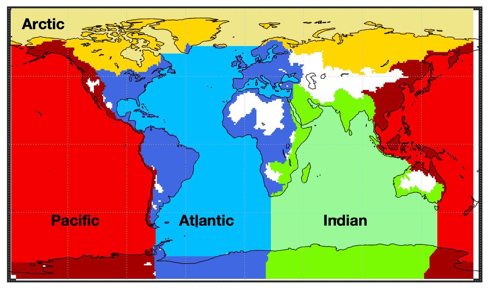
Figure 1The Pacific, Atlantic, Indian, and Arctic ocean basins and their associated continental drainage basins according to the global continental runoff pathways scheme of Oki and Sud (1998). Within each basin, the darker colour represents the continental basin, and the lighter colour represents the ocean basin. White regions represent endorheic basins.
2.2 Precipitation and evaporation data
The P and E data that we use are adopted from the ERA5 reanalysis (Hersbach et al., 2018), which assimilates observations into general-circulation modelling provided by the European Centre for Medium-Range Weather Forecasts (ECMWF). They are given at 0.25∘ latitude–longitude regular grids and monthly (and hourly) intervals for global coverage of both continents and oceans. In order to match the spatial resolution of the above-mentioned continental runoff pathways data, we homogenize the grid to by averaging the corresponding 0.25∘ grid points.
2.3 Time-variable GRACE data
The critical knowledge needed in Eqs. (1) and (2), which is now obtainable from GRACE monthly data, is dW (Tapley et al., 2004, 2019) – the month-to-month difference in the stored water. Note that the GRACE mass variability pertains directly to WT, as opposed to, for example, altimetric sea level measurements that also contain non-WT, steric effects. We use the GRACE “mascon” (mass concentration) solutions that have already been converted into surficial mass from the original time-variable gravity observations (in our case, the GRACE RL06 mascon dataset provided by the Center of Space Research, CSR, of University of Texas; see Save et al., 2016; Save, 2019). The non-surficial gravity change due to the glacial isostatic adjustment (GIA) has been removed to the extent of the ICE6G-D model (Peltier et al., 2018). Any other non-surficial effect such as long-term tectonics would be incorrectly interpreted as water-mass fluxes (Chao, 2016), but they may only be important in the determination of secular trends. Additional non-climatic sources, such as the rare local earthquake events, may be similarly misinterpreted. As the C20 Stokes coefficient is not well determined from the GRACE mission, it is replaced by a more accurate solution from satellite laser ranging (SLR; Cheng and Ries, 2017). GRACE is not sensitive to geocenter variations, and its degree-1 Stokes coefficients are set to zero. We tried adding an estimate of geocenter variations due to modelled water-mass variability to GRACE data (Swenson et al., 2008) and found that our reported results only changed by less than 1 %. Furthermore, the atmospheric effects as well as some oceanic effects on gravity change have already been removed from the processing of the GRACE data by CSR, for de-aliasing purposes, according to the operational numerical weather prediction (NWP) model from ECMWF and to an unconstrained simulation with the global ocean general circulation model MPI-OM (Max-Planck-Institute Global Ocean/Sea-Ice Model; Dobslaw et al., 2017). To recover the “true” ocean mass variability, we restore the removed signal on the oceans by adding back the GAD product, which is set to zero on the continents. Data are provided on a 0.25∘ regular grid; we reduce the resolution to 1∘ regular grids, which is still finer than the spatial resolution of GRACE (∼300 km), in order to match the spatial resolution of the continental drainage basin data as above.
GRACE's degree-0 Stokes coefficients ΔC00 are set to be identical to zero on the basis that Earth's total mass (including the atmosphere) is constant. Any increase (decrease) in the water-mass budget of the atmosphere will then be counteracted by a decrease (increase) of the same amount of water mass at the surface. However, after the atmospheric and dynamic oceanic mass changes are corrected for in GRACE data, the GRACE ΔC00 values are still set to zero, even though they should match the opposite of the removed signals. To restore the lost degree-0 signal, the GAD product (which is set to zero on the continents) must be added back to GRACE with the averaged ocean signal set to zero; the ΔC00 from an atmospheric model must then be subtracted from GRACE data in order to force the Earth's total mass to be constant. After these steps have been undertaken, the GRACE data will account for the global exchange of water mass between the Earth surface and the atmosphere. Such a correction has recently proven to improve the agreement between the GRACE global ocean mass change and non-steric sea level variation estimates from altimetry and ARGO data (Chen et al., 2019). Looking for consistency between the GRACE and ERA5 datasets, we use ΔC00 from P−E to restore the degree-0 signal in dW. This ΔC00 accounts for uniform mass variations in the global surface that are equivalent to a global averaged signal for P−E, at 188 Gt per month (95 % confidence interval CI95=[136, 243], see below). As global represents the variability of global total-column water (TCW), it should match the time derivative of the global TCW. However, the average rate of change in the global TCW in ERA5 is 1.5 Gt per month (CI, 12.7]); although this is in the range of previously reported values of [−0.9, 4.3] Gt per month (Nilsson and Elgered, 2008), it is far removed from the global value. This reveals some internal inconsistency within the ERA5 dataset. However, while this artificially increases the dW estimate, the excessive value of P−E does not affect the WT components R and N estimated from Eqs. (1) and (2), as the degree-0 signal vanishes due to the residual estimate between dW and P−E. In fact, adding ΔC00 from P−E to GRACE is numerically equivalent to setting P−EΔC00 to zero as far as Eqs. (1) and (2) are concerned.
2.4 Confidence intervals
The reported 95 % confidence intervals and the correlation coefficients are evaluated using the stationary bootstrap scheme of Politis and Romano (1994) (with the optimal block length selected according to Patton et al., 2009) as well as the percentile method. The intuition underlying the bootstrap scheme is simple. Suppose that the observed time series x1, …, xn is a realization of the random vector (X1, …, Xn) with the joint distribution Pn and which is assumed to be part of a stationary stochastic process. Given Xn=(X1, …, Xn), we first build and estimate of Pn. B random vectors (, …, ) are then generated from . If is a good approximation of Pn, the relation between (, …, ) and should reproduce the relation between (X1, …, Xn) and Pn well (for an introduction to bootstrap methods for time series, see Kreiss and Lahiri, 2012, and the references therein). Here, the number of bootstrap replications was set to B=2000. In general, the half-length of the confidence interval can be approximated very well by twice the standard deviation of the sample mean estimated from the bootstrap replications. Prior to applying the bootstrap to a time series, the least-squares estimated linear and quadratic trend as well as the sinusoid with the most relevant frequencies are removed from the series to meet the stationarity conditions of the method. In particular, each series has been decomposed into trend, seasonal, and residual components. The bootstrap is applied to the residual component and produces bootstrap samples of the residuals. For the evaluation of confidence intervals for the different components of WT, the trend and seasonal terms are added back (to the bootstrap sample of the residuals), producing bootstrapped time series of the component of interest. These samples are then used for further analysis. As an illustration, for the WT N component, we proceed as follows: (i) a model with linear, annual, and semiannual signals is fitted to the data, and the fitted linear trend and the annual and semiannual signals are subtracted from the original time series; (ii) the stationary bootstrap is then applied to the residuals, producing 2000 bootstrap samples of the residuals; (iii) the estimated trend and seasonal components are added back to each bootstrap sample of the residuals which results in an ensemble of 2000 bootstrapped time series for the N component; (iv) these 2000 bootstrapped time series are used to obtain the 95 % confidence intervals for the mean fluxes (average of N over the 14-year period of study) and for the amplitude and phase of the annual component using the percentile method. For the mean fluxes, the average of N for each of the 2000 bootstrapped time series was first evaluated, and the 0.025 and 0.975 percentiles of these 2000 averages were then reported as the 95 % confidence interval. For the study of the climatology, a linear trend model with annual and semiannual components was fitted to the 2000 bootstrapped time series, producing corresponding estimates of the annual amplitude and phase. The 0.025 and 0.975 percentiles of these estimates were reported as the 95 % confidence intervals. In order to study the robustness of the results with respect to the model choice, the analysis is rerun using 11 alternative models that are obtained by considering different forms of the trend component (quadratic or constant) and including higher frequencies in the harmonic regression (up to 5). The results are robust. The relative difference with respect to the reported values is less than 1.2 % for point estimates and less than 3.3 % for the extremes of the 95 % confidence intervals.
As an independent check of the bootstrap, confidence intervals for the mean value of N have been also evaluated by propagating the error estimate in GRACE data (using the JPL GRACE mascon solution for which error estimates are available). The resulting intervals were consistent with those of the bootstrap method. In particular, we show that, in all cases, the bootstrap intervals contain the intervals obtained from error propagation (see Sect. 4 for details). In this respect, the CI95 from bootstrap analysis can be considered a conservative estimate. This should be expected, as the residual component underlying the bootstrap approach includes measurement errors and other type of errors (related, for example, to the estimate of the trend and seasonal terms). As a result, the uncertainties in the transports estimated by the bootstrap should be larger than the corresponding uncertainties estimated by error propagation.
Note that the bootstrap was applied to the bivariate time series of the residuals of the two variables of interest for the study of correlation, producing an ensemble of 2000 bivariate time series of residuals. For each bivariate time series of residuals, the correlation between the two components of the series was first evaluated. The average and the 0.025 and 0.975 percentiles of these 2000 estimates were reported as a point estimate and confidence limits respectively for the correlation between the two variables of interest (the correlation between the residual components is used to avoid spurious correlation).
The various WT components of the Pacific and its associated land drainage regions are shown in Fig. 2 in units of gigatonnes per month (1 Sv ≈ 2600 Gt per month; 1 Gt = 1012 kg, the weight of 1 km3 of freshwater). The same analysis is applied to the rest of the ocean basins, i.e. to the “non-Pacific” AIA oceans, individually and collectively, with their associated land drainages (see Fig. 1).
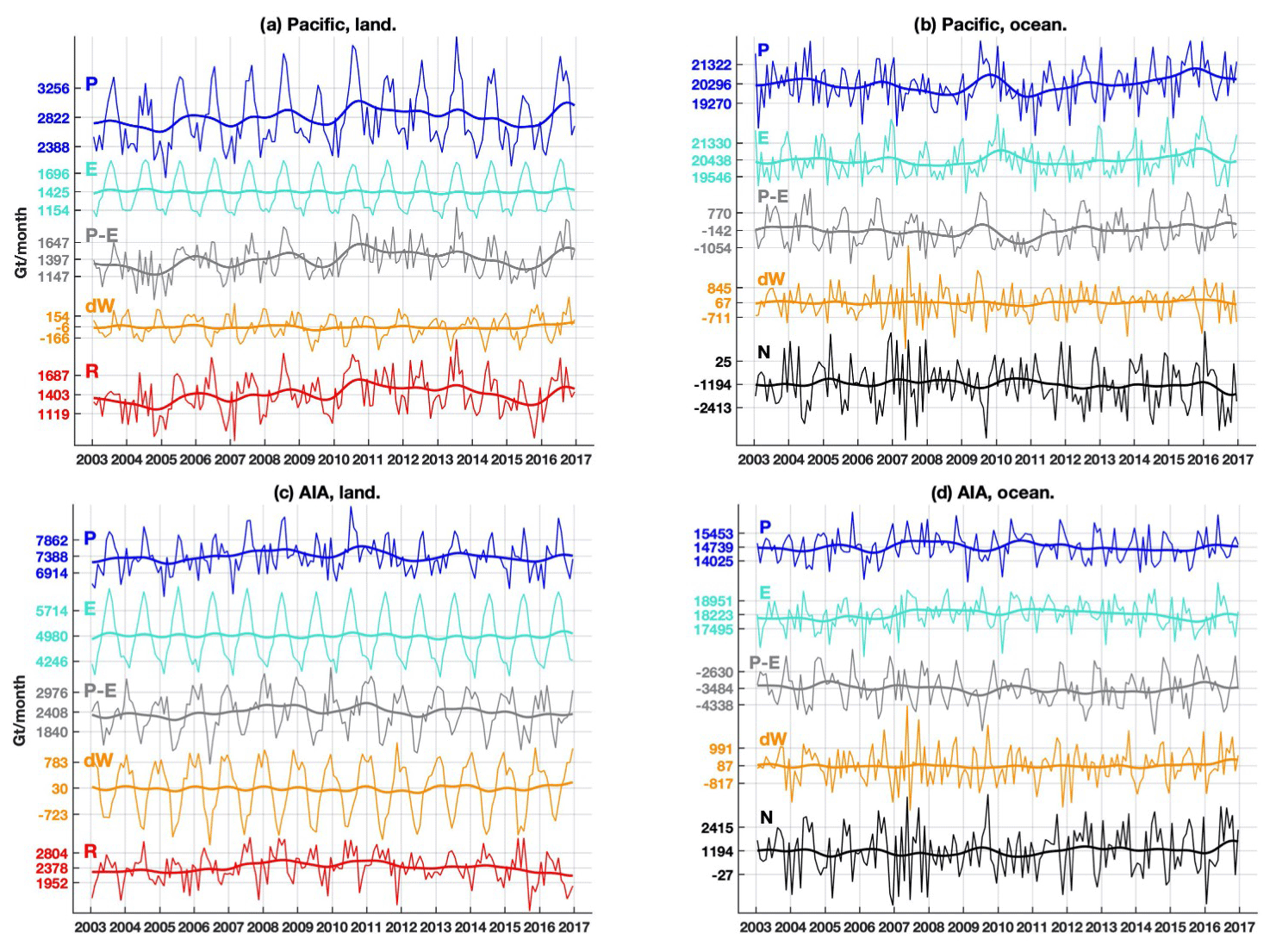
Figure 2WT from Eqs. (1) and (2) in the Pacific (a, b) and in the Atlantic, Indian, and Arctic (AIA) oceans collectively (c, d), as well as their drainage basins. (a, c) The associated land drainage basins and (b, d) ocean basins. Labels on the y axis correspond to the mean ± standard deviation of the associated curve. Thick lines are the low-pass-filtered signal by a Hann function of 24 months. All curves in the same panel are plotted on the same scale. P, E, and P−E are from the ERA5 dataset; dW is estimated from GRACE; R and N are estimated as a residual in Eqs. (1) and (2) respectively.
3.1 Mean fluxes
Averaged over the 14 years studied, the Pacific Ocean loses water through the atmospheric P−E at an average rate of 142 Gt per month (CI95=[48, 243]), which is greatly overcompensated for by an inflow R from land of 1403 Gt per month (CI95=[1370, 1436]). From this surplus, a minor (if any) amount of 67 Gt per month (CI95=[25, 108]) remains (and accumulates) in the Pacific, while 1194 Gt per month (CI95=[1096, 1291]) is transported horizontally to the “non-Pacific” Atlantic, Indian, and Arctic (AIA) oceans, which will be referred to as the “Pacific outflow” hereafter.
In the AIA oceans, the situation is found to be markedly distinct, given the fact that the AIA oceans have a combined surface area comparable to the Pacific (177×106 km2). The AIA oceans collectively lose 3484 Gt per month (CI95=[3406, 3560]) through the atmospheric P−E, which is ∼25 times the amount lost by the Pacific. Only ∼68 % of this water deficit is compensated for by a land R inflow of 2378 Gt per month (CI95=[2337, 2419]). With the nominal minor amount of water accumulation of 87 Gt per month (CI95=[44, 130]), the AIA oceans consequently present an average inflow of 1194 Gt per month (CI95=[1102, 1284]) from the Pacific, which will be referred to as the “AIA inflow” hereafter.
As expected from the overall conservation of water mass inherent in our methodology, the estimated Pacific outflow and the AIA inflow match (Fig. 3). It is worth mentioning that a difference of 188 Gt per month would exist between the two mean flux values if the degree-0 correction was not applied.
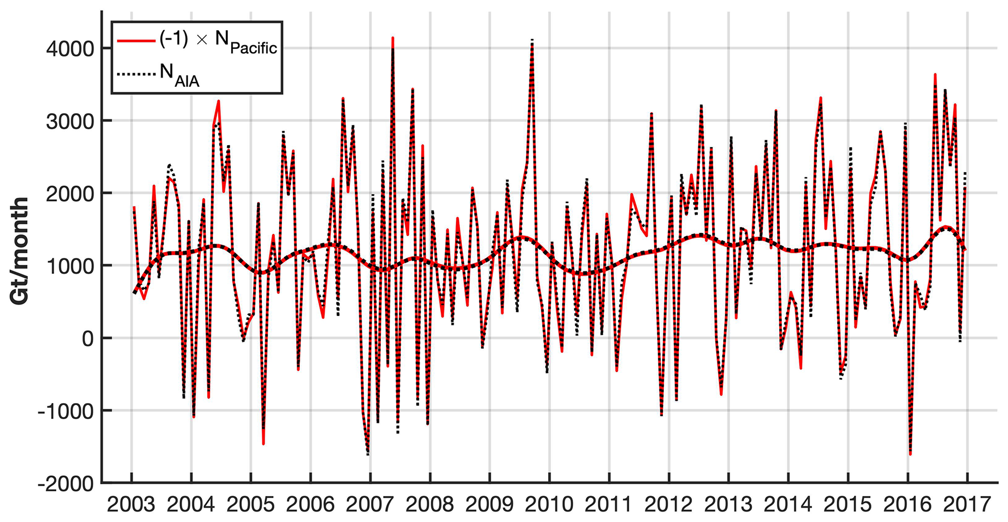
Figure 3Monthly time series of WT flux from the Pacific to the AIA oceans. The red curve is (the opposite of) the Pacific outflow, and the black curve is the AIA inflow. Thick lines are the low-pass-filtered signal by a Hann function of 24 months.

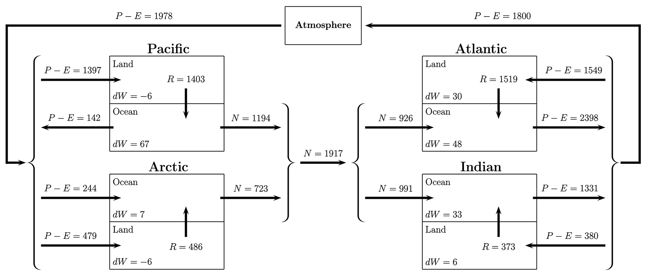
Figure 5Diagram of the mean values of the WT of the study regions. Units are in gigatonnes per month.
Corresponding analyses have been performed for the Atlantic, Indian, and Arctic oceans separately. The time evolution of the WT components in Eqs. (1) and (2) are shown in Fig. 4, and a diagram of the water-mass fluxes is shown in Fig. 5. On average, the Atlantic Ocean receives 926 Gt per month (CI95=[876, 980]; or 0.36 Sv) of salty water, and it loses 879 Gt per month (CI95=[828, 930]) to the atmosphere via . The latter is equivalent to a freshwater deficit of 0.34 Sv, which increases the near-surface salt concentration and enables water to sink in the North Atlantic, producing deep water. These values are close to the 0.13–0.32 Sv estimated from ocean models, as needed to maintain the salinity balance in the Atlantic Ocean (Zaucker et al., 1994). Similarly, the Indian Ocean loses 957 Gt per month (CI95=[894, 1022]) of freshwater that is restored by 991 Gt per month (CI95=[907, 1073]) of salty water. The freshwater lost by the Atlantic and Indian oceans via goes to the Pacific (1261 Gt per month, CI95=[1171, 1347]) and Arctic (730 Gt per month, CI95=[712, 747]) oceans, which return 1194 (CI95=[1096, 1291]) and 723 (CI95=[708, 739]) Gt per month of salty water through the ocean respectively. Thus, the Pacific presents a surplus of freshwater that reduces the near-surface salt concentration, preventing the formation of deep water. Together, the Pacific and Arctic oceans supply 1917 Gt per month (CI95=[1812, 2021]) of water to the Atlantic and Indian oceans, where it is reincorporated into the water cycle via net E−P. As in previous studies (see Craig et al., 2017, for a synthesis), the freshwater lost in the Indian Ocean is similar to that in the Atlantic Ocean. In these studies, is close to zero in the Pacific Ocean, producing a difference of 0.4 Sv between the Atlantic and Pacific oceans. In our study, is 1261 Gt per month in the Pacific Ocean, and the difference with the Atlantic increases to ∼0.8 Sv. Some of these differences would be expected, as the ocean basins are not defined in exactly the same way. On the other hand, the global R is 3781 Gt per month (or km3 yr−1), which is close to the 41 867 km3 yr−1 reported by the Global Runoff Data Centre (GRDC, 2014). At the basin scale, R is 16 834 km3 yr−1 in the Pacific, which is greater than the 11 826 km3 yr−1 reported by GRDC. In the Atlantic, Indian, and Arctic, R is 18 228, 4479, and 5827 km3 yr−1 respectively, which is closer to the respective GRDC values of 20 772, 5238, and 4080 km3 yr−1. Finally, according to the diagram in Fig. 5, the water content in the atmosphere decreases by 178 Gt per month (and is gained by Earth's surface), but this amount is not realistic (as discussed in Sect. 2), as it should increase by a few gigatonnes per month (Nilsson and Elgered, 2008). This value differs from the 188 Gt per month mentioned in Sect. 2 because the endorheic regions are not considered here.
3.2 Annual climatology
The WT climatology of the N component is estimated in two ways: (1) averaging the 14 N values for each month of the year (Fig. 6a) and (2) fitting a linear trend as well as annual and semiannual components' model as described in Sect. 2. Annual amplitudes and phases are plotted in Fig. 6b and reported, with their corresponding 95 % quantile-based confidence intervals, in Table 1.
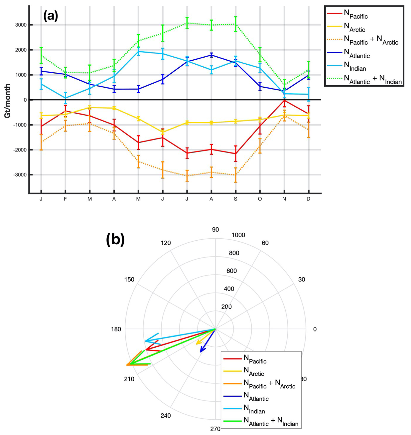
Figure 6(a) Annual climatology time series (the error bar is 1 standard deviation) and (b) phasor diagram (amplitude in units of Gt per month, phase angle according to Eq. 3) of the inflow and outflow WT of the ocean basins.
Table 1Mean and annual signals of the N component as estimated from the CSR mascon solution for different ocean basins according to Eq. (2).
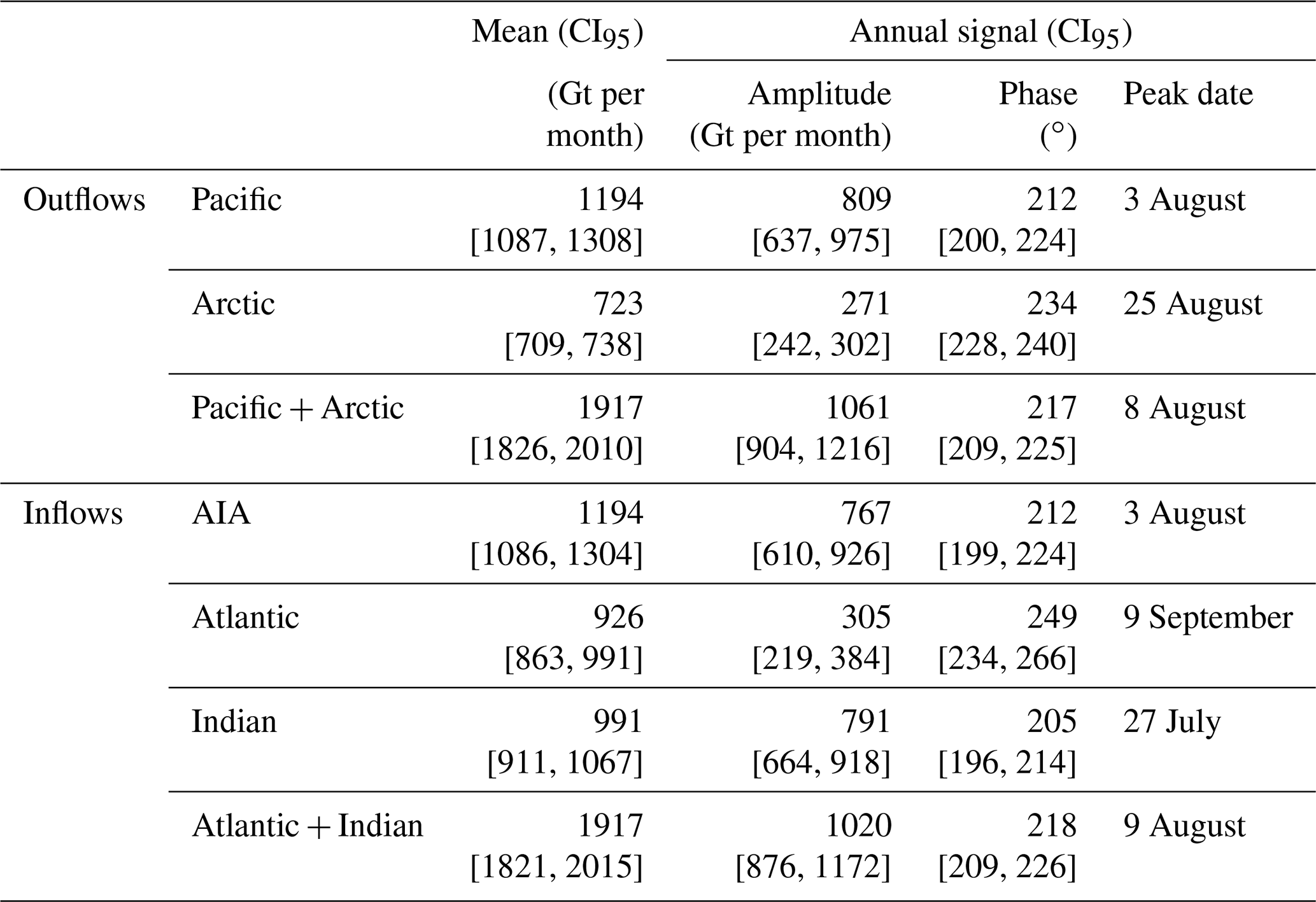
The Pacific and Arctic oceans show an overall outflow throughout the year; this is in contrast to the Atlantic and Indian oceans, which show an inflow for every month. The Pacific outflow shows a prominent seasonal undulation that peaks around 3 August and a peak-to-peak WT variation of ∼2000 Gt per month from boreal summer to November, when a near-zero minimum occurs. The Arctic Ocean shows half of the Pacific variability and a less pronounced seasonal undulation. A minimum outflow of ∼320 Gt per month is reached in March and April, and a maximum outflow of ∼1300 Gt per month is seen in July. Together, the Pacific and Arctic oceans send ∼3000 Gt per month of seawater to the Atlantic and Indian oceans during boreal summer and a minimum amount 5 times lower (around 600 Gt per month) in November. The annual maximum is reached on 8 August. The combination of the Atlantic and Indian inflow mirrors this behaviour. The respective Atlantic and Indian inflows show a similar peak-to-peak variation of ∼2000 Gt per month, reaching their respective maxima in August and May. The Indian maximum seems to be related to a local maximum of the Pacific outflow. The annual maxima of the net WT of the four basins are reached between 3 August and 9 September, although the annual signals of the Pacific and Indian oceans are almost triple those from Arctic and Atlantic oceans (Table 1 and Fig. 6b).

Figure 7Pacific outflow and climatic indices for ENSO, AMO, AO, and AAO. (a) The time series of the Pacific outflow is de-trended and de-seasonalized. All time series are normalized to have unit variance. Values in parenthesis are the correlation coefficients between the corresponding climatic index and the Pacific outflow. (b) Correlation coefficients between de-trended and de-seasonalized WT components of different regions and the climatic indices.
3.3 Interannual variability
Interannually, the Pacific outflow shows remarkable variability, mainly produced by P on the continents, which is inherited by R, and P−E in the oceans (Fig. 2). For example, the Pacific outflow shows a maximum of around 1372 Gt per month in 2009 that matches with a P−E maximum in the Pacific, a P−E minimum in the AIA oceans, and P minima in the continental basins draining to both the Pacific and AIA oceans. The opposite behaviour, a minimum of around 939 Gt per month, is observed in 2010. The difference, 433 Gt per month, is comparable to the discharge from the Amazon (Lorenz et al., 2014). In the tropical Pacific, the El Niño–Southern Oscillation (ENSO) is the strong recurring climate pattern involving changes in the temperature of seawater and air pressure in the tropical Pacific Ocean. ENSO had a mild El Niño phase in 2009 followed by a strong La Niña phase in 2010, which may be related to the interannual variability of the Pacific outflow. To elucidate this, we conduct a correlation study of the interannual Pacific outflow with respect to the major climate oscillations in the Earth's atmosphere and ocean: ENSO, the Atlantic Multi-decadal Oscillation (AMO), the Antarctic Oscillation (AAO), and the Arctic Oscillation (AO). The climatic oscillation is represented by monthly time series of its indices, which are non-dimensional functions of time derived from relevant meteorological observations; their values indicate the polarity and strength of the oscillation at a given epoch. The ENSO oscillations are measured here with the Southern Oscillation index (SOI), which represents the sea level pressure differences between Tahiti and Darwin, Australia. The AMO is a coherent mode of natural variability based upon the average anomalies of sea surface temperatures, with the AMO index reflecting the non-secular multi-decadal sea surface temperature pattern variability in the North Atlantic basin. The AAO describes the intensity of the westerly wind belt surrounding the Antarctic, quantified by the AAO index, which is the leading principal component of the 700 hPa atmospheric geopotential height anomalies poleward of 20∘ S. The AO is to be interpreted as the surface signature of modulations in the strength of the polar vortex aloft in the Arctic, and the AO index is constructed by projecting the 1000 hPa height anomalies poleward of 20∘ N. Figure 7a shows all of the indices with the amplitudes normalized to 1 standard deviation, as well as the de-trended, de-seasonalized, standard-deviation-normalized Pacific outflow. The correlation analysis between the Pacific outflow and the SOI shows no overall correlation (Pearson coefficient of 0.03) during the whole period, meaning that the influence of ENSO on the Pacific outflow may be restricted to the strong ENSO phases, such as in 2009 and 2010. A similar lack of correlation (lower than 0.1) is observed with respect to the AMO, AAO, and AO.
To explore this lack of correlation, we have estimated the correlation coefficient between each climatic index and each WT component (Fig. 7b). All of them are lower than 0.3 except for six cases in two regions. In the Arctic, P and P−E in the drainage basins of the Arctic show a correlation of ∼0.5 with the AO. This correlation is natural, as the Arctic is the area that influences the AO. The other region is the Pacific, where, as expected, the SOI shows a correlation of around 0.5 with P, P−E, and R in the drainage basins, and of around −0.4 with P in the ocean. However, this individual correlation does not extend to the Pacific outflow. In order to understand why this is the case, it is convenient to express the N component of the water transport as a function of P−E and dW. According to Eqs. (1) and (2), we have
The correlation between N and a given index can then be express as follows:
where corr denotes the correlation coefficient, and SD stands for standard deviation. As shown in Eq. (4), the correlation between N and a given index is a linear combination of the correlation between each component and the index. The coefficients of the linear combination, SD(Xi)∕SD(N) are proportional to the standard deviation of each component. The components of Eq. (4) for the Pacific outflow and the SOI index are shown in Table 2. Despite the fact that some of the individual components exhibit significant correlations with SOI (in particular P−E in land and ocean), when they are combined with the corresponding coefficients, their effects cancel out, yielding a negligible correlation between water transport and SOI (below 0.03 in magnitude). Note that Table 3 also provides some insights into the causes of the interannual variability of Pacific Ocean outflow. The largest standard deviation of P−E and dW in the ocean suggests that these two components might drive the interannual variability of the Pacific Ocean outflow. This is confirmed by a correlation analysis. The correlation between N and (P−E)ocean is −0.70. The correlation between N and dWocean is 0.84. The correlation between N and the corresponding land components is below 0.18. In all cases, the corresponding time series have been de-trended and de-seasonalized prior to the evaluation of the correlation.
Another possible reason for the lack of correlation resides in the definition of the study regions, for which the presence of subregions with a positive and negative influence from an index results in an overall negligible or attenuated influence of the index in the overall region. For example, a positive phase of the AMO is related to an increase in P in western Europe (Sutton and Hodson, 2005) and the Sahel (Folland et al., 1986; Knight et al., 2006; Zhang and Delworth, 2006; Ting et al., 2009), but to a decrease in P in the US (Enfield et al., 2001; Sutton and Hodson, 2005) and northeast Brazil (Knight et al., 2006; Zhang and Delworth, 2006). All of these regions are included in the Atlantic drainage basin, and the influence of a positive phase of the AMO is then attenuated.
In this section, we perform a comparison using alternative datasets. In particular, we implement the following changes:
-
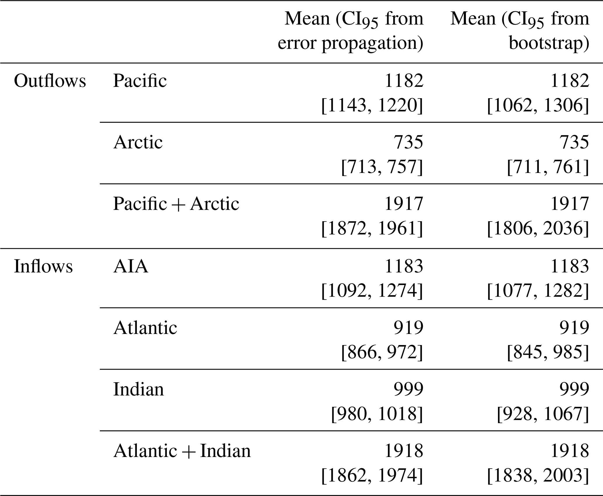
the CSR GRACE mascon solution is replaced by the JPL GRACE mascon solution provided by the NASA Jet Propulsion Laboratory (Watkins et al., 2015; Wiese et al., 2019). Similarly to the CSR data, JPL data are corrected for GIA effects, the C20 Stoke coefficients are replaced by a solution from SLR, and data are reduced to 1∘ regular grids from 0.5∘ regular grids. In addition, we applied the degree-0 Stoke coefficients correction. However, CSR and JPL mascon solutions are not directly comparable. The main reason for this is that an estimate of degree-1 coefficients has been added to JPL mascon solutions, and the GAD product has not been added back. The corrections applied by JPL are not supplied separately; thus, we cannot do or undo any of the corrections to process the JPL data as we did with CSR data. In particular, the GAD product is not available for JPL. In any case, the JPL solution is useful here, as it provides an error estimate of the mascon solution that can be propagated to obtain confidence intervals of N, which are independent of those estimated with the bootstrap analysis. Table 3 shows the CI95 of the mean values of the N component estimated from error propagation and bootstrap analysis for the different ocean basins. In all cases, it is observed that the CI95 values from error propagation are included in those from bootstrap analysis, meaning that the CI95 values from the bootstrap analysis are a conservative estimate of the error. The JPL propagated error can be expected to be similar to that propagated from CSR error estimates (which are not available); thus, we can assume that the reported CI95 values for N calculated from CSR data are a conservative estimate. In addition, comparing Tables 1 and 3, it is observed that the mean values of N are quite similar and that the CI95 values largely overlap. Regarding the time variability, the values of the N component from the CSR and JPL mascon solutions show Pearson correlation coefficients greater than 0.85 (p value < 10−3), except for the Atlantic (0.70). Thus, despite the different processing methods used for CSR and JPL data, the reported analysis for the N component is robust with respect to the choice of GRACE datasets.
-
ERA5 P and E data are replaced by several datasets for comparison purposes. The objective is not to be exhaustive in the selection, but rather to show that the reported features of the N component are quite robust with respect to the choice of the P and E datasets. The datasets considered are:
- i.
continental P from GPCC (Schneider et al., 2011), GPCP (Adler et al., 2018), CMAP (Xie and Arkin, 1997), UDel (Willmott and Matsuura, 2001), and GLDAS/Noah (Rodell et al., 2004; Beaudoing and Rodell, 2016);
- ii.
ocean P from GPCP and CMAP;
- iii.
continental E from GLEAM (Miralles et al., 2011; Martens et al., 2017) and GLDAS/Noah;
- iv.
ocean E from OAFlux (Yu et al., 2008) and HOAPS/CM SAF (Schulz et al., 2009).
- i.
The Pacific outflow is estimated using the 162 possible combinations of P and E, including ERA5. The time period used is from 2003 to 2016, except for HOAPS/CM SAF and GPCP, which span from 2003 to December 2014 and October 2015 respectively. The degree-0 corrections in the GRACE data is made for each combination. Note that only ERA5 includes P and E for both continents and oceans. All grids have been homogenized to 1∘ regular grids. The main concern here is the heterogeneity of the spatial coverage among datasets. To make the results comparable among datasets, the computations are restricted to the common grid points, which do not cover the entire Earth (Fig. 8a). However, in spite of the fact that the principle of water-mass conservation is not fulfilled due to the partial coverage, the Pacific outflow obtained in the common grid points from ERA5 (black line in Fig. 8b) is in quite good agreement with the same signal obtained with global coverage (the red line in Fig. 3, which is also reported as the red line in Fig. 8b). The Pearson correlation coefficient between the two signals is 0.994 (p values < 10−3) with an average difference of around 50 Gt per month. In general, the Pacific outflows estimated from all of the P and E dataset combinations show qualitatively the same signal as the one reported in Fig. 3. For each of the 162 estimates of the Pacific outflows corresponding to the possible P and E dataset combinations, we evaluated the average outflow (over the period of study), which is 968 Gt per month (SD of 489), and the correlation with the Pacific outflows in Fig. 3, which is 0.82 (SD of 0.06; p values < 10−3).
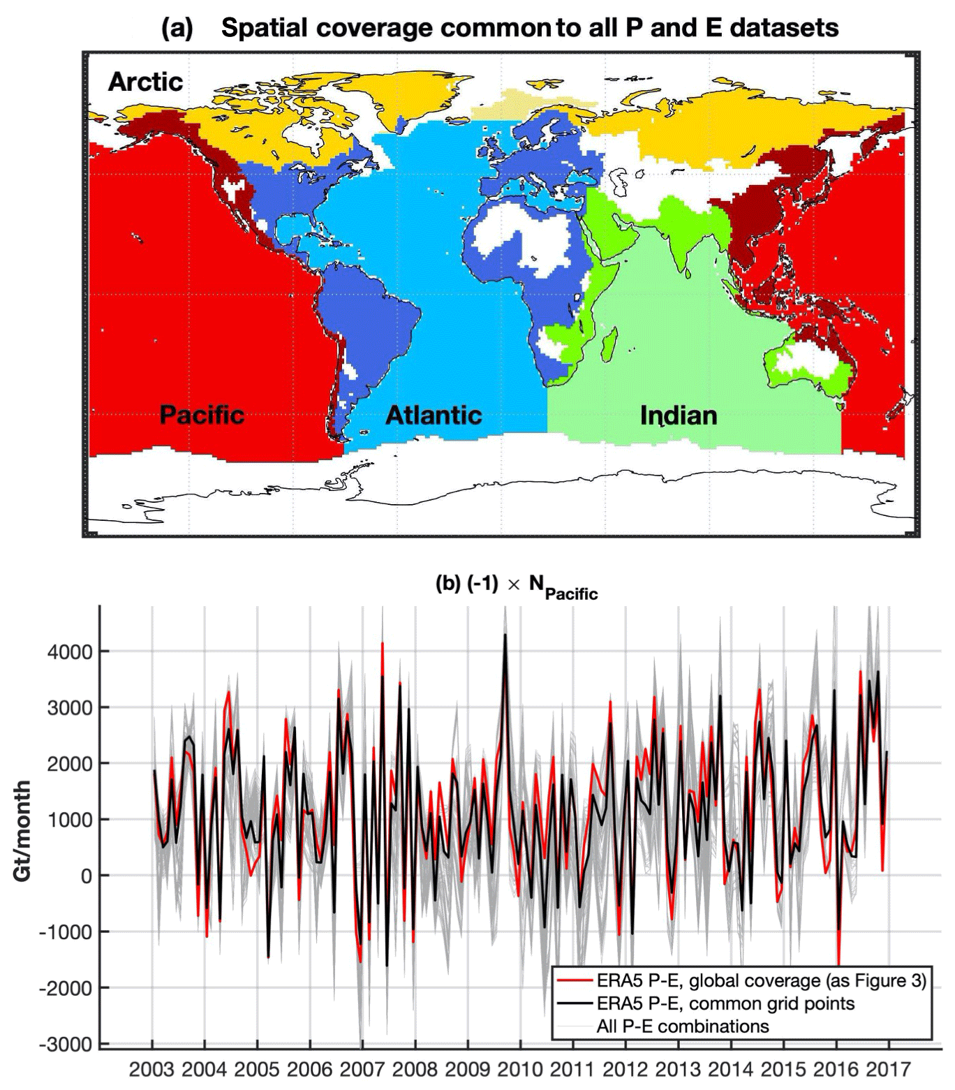
Figure 8Monthly time series of (the opposite of) the Pacific outflow estimated from 162 combinations of P and E datasets. (a) Spatial coverage common to all datasets. (b) Pacific outflows: grey thin curves are the 162 Pacific outflows estimated in the grid points common to all datasets (no global coverage); black and red curves are based on ERA5 P and E and are obtained using either only the grid points common to all datasets (black curve) or global coverage (red curve). Note that the red curve is the same as in Fig. 3.
Table 2Correlation coefficients between the SOI and the de-trended and de-seasonalized WT components involved in the estimate of the Pacific outflow according to Eqs. (3) and (4).
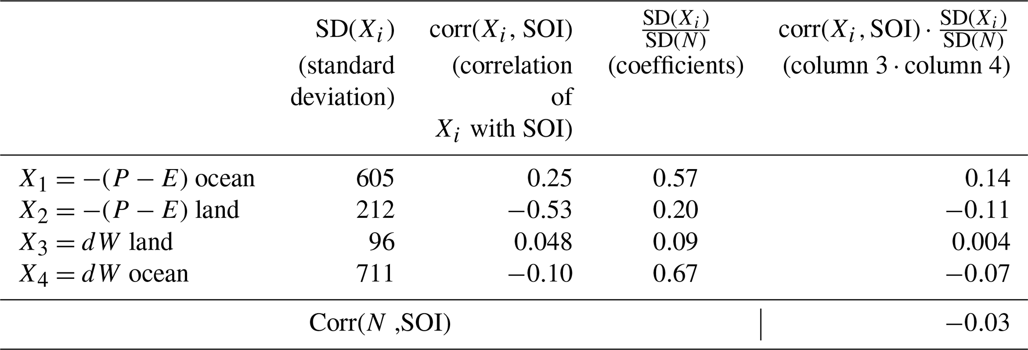
Table 3Mean of the N component as estimated from the JPL mascon solution for different ocean basins according to Eq. (2). CI95 values are estimated as the propagation of mascon errors provided by JPL and from bootstrap analysis. Units are gigatonnes per month.
These experiments show that the reported net WT values are physically consistent among datasets, at least qualitatively.
In this work, we present a new methodology that combines GRACE data with the general hydrologic budget equation to estimate the horizontal water-mass convergence and divergence for any oceanic region. We have assumed that the gravity changes are produced by mass changes on the Earth surface, such as in the oceans, so that the mascon solution is physically meaningful (Chao, 2016). Any mis-modelling of the ocean basin “container” volume change due to GIA and other non-surficial changes would masquerade as WT variations. However, they are not critical as far as our non-secular analysis is concerned.
We use the proposed methodology to estimate the net WT and exchanges among the Pacific, Atlantic, Indian, and Arctic oceans, for the period from 2003 to 2016. Our main finding is that the Pacific and Arctic oceans, while replenished with precipitation and land runoff, are nearly continuously losing water to the Atlantic and Indian oceans. In particular, the WT climatology is such that the Pacific Ocean loses water at a rate from near zero up to the peak of 2000 Gt per month during the boreal summer, which coincides with the maximum of the global atmosphere water content. On top of the climatology, the interannual Pacific annual mean water loss varies significantly between ∼950 and ∼1450 Gt per month during the study period, but this is seemingly uncorrelated with ENSO.
The results presented here are consistent with the well-known salinity asymmetry between the Pacific and Atlantic oceans (Reid, 1953; Warren, 1983; Broecker et al., 1985; Zaucker et al., 1994; Rahmstorf, 1996; Emile-Geay et al., 2003; Lagerloef et al., 2008; Czaja, 2009; Reul, 2014). However, they are in contrast to previous GRACE-based studies where a simple see-saw WT between the Pacific and the Atlantic and Indian oceans has been reported (Chambers and Willis, 2009; Wouters et al., 2014). In those studies, the term in Eq. (2) in both the Pacific and the Atlantic and Indian oceans was approximated by that from the global ocean mean. However, the mean freshwater flux in the Pacific (1261 Gt per month) does not really match with that in the Atlantic and Indian oceans (−1837 Gt per month), meaning that the approximation was quite poor; hence, the N term was not properly estimated in these studies (see the Appendix for further discussion).
Differences in freshwater fluxes between the Pacific and Atlantic oceans produce salinity contrasts and, in turn, differences in deep water formation. Nevertheless, there are other factors influencing these contrasts such as the narrower extent of the Atlantic (de Boer et al., 2008; Jones and Cessi, 2017), the meridional span of the African and American continents (Nilsson et al., 2013; Cessi and Jones, 2017), and the salty WT from the Indian Ocean to the Atlantic (Gordon, 1986; Marsh et al., 2007). The AMOC is also influenced by WT through the Bering Strait (Reason and Power, 1994; Goosse et al., 1997; Wadley and Bigg, 2002) as well as by the surface processes of temperature, precipitation, and evaporation at low latitude in the Pacific and Indian oceans (Newsom and Thompson, 2018). The relative importance of the multiple drivers influencing the AMOC is an open problem (Ferreira et al., 2018). The net WT estimated here provides information on differences between oceanic inflows and outflows, which can be useful to help clarify this problem.
Net WT in the open oceans can alternatively be estimated using global ocean models, which simulate observational data based on physical principles. However, these models are not necessarily sensitive to the WT, especially given the data types and the geographical and topographical resolutions involved in the models. Knowledge about three-dimensional global ocean circulation could also elucidate the net WT. However, the small ratio between the net and the total WT hinders the estimation of the former from the latter.
We have applied our WT estimation scheme to the four major ocean basins. The methodology can of course be applied to any extensive ocean region of interest as long as it is much larger than the GRACE resolution. The findings reported here will be useful for a better understanding of the global climate system in terms of its climatology and spatio-temporal variations.
We shall show here that the net water-mass exchange between the Pacific and the Atlantic and Indian oceans reported by Chambers and Willis (2009) was a mathematical artefact. Their Eq. (2) approximated the freshwater flux, i.e. , of the Pacific (Pcf) and the Atlantic and Indian (AI) oceans using the global ocean (GO) mean. However, from Figs. 2 and 4, we get very different results, ( and ( Gt per month, meaning that the approximation in Chambers and Willis (2009) and, hence, their resultant estimates of WT are rather poor. In addition, using their approximation, an apparent net mass exchange will always arise, as
where x are disjoint grid cells in the ocean basins; the areas of the Pcf, AI, and GO are around 177, 160, and 351×106 km2; and the ratios 177∕351 and 160∕351 have been approximated by 1∕2. Then, multiplying by 2 and rearranging the equation, we get
Thus, wherever the signal is in the Pacific and the Atlantic and Indian oceans, the anomalies with respect to the global ocean mean will always mirror each other, showing an apparent net mass exchange between them, even if such an exchange does not exist.
We thank the organizations that provide the data used in this work, which are publicly available: ERA5 data are provided by the Copernicus Climate Data Store (CDS), https://cds.climate.copernicus.eu/cdsapp#!/home (last access: 30 April 2019) (Hersbach et al., 2018); GPCC (Schneider et al., 2011), CMAP (Xie and Arkin, 1997), and UDel (Willmott and Matsuura, 2001) precipitation data are provided by the NOAA/OAR/ESRL PSD, Boulder, Colorado, USA, https://www.esrl.noaa.gov/psd/ (last access: last access: 27 May 2019); GPCP precipitation data are provided by the Mesoscale Atmospheric Processes Laboratory, NASA Goddard Space Flight Center, https://precip.gsfc.nasa.gov/ (last access: 13 June 2019) (Adler et al., 2018); OAFlux evaporation data are provided by the WHOI OAFlux project (http://oaflux.whoi.edu, last access: 28 May 2019) (Yu et al., 2008), funded by the NOAA Climate Observations and Monitoring (COM) programme; HOAPS evaporation data are provided by CM SAF/EUMETSAT, https://www.cmsaf.eu (last access: 28 May 2019) (Schulz et al., 2009); GLDAS/Noah data are provided by GSFC/NASA, https://disc.gsfc.nasa.gov/ (last access: 28 May 2019) (Rodell et al., 2004; Beaudoing and Rodell, 2016); GLEAM evaporation data are available at https://www.gleam.eu/ (last access: 27 May 2019) (Miralles et al., 2011; Martens et al., 2017); GRACE time-variable gravity data are provided by CSR, University of Texas, http://www2.csr.utexas.edu/grace (last access: 16 July 2019) (Save et al., 2016; Save, 2019), and by JPL/NASA, https://podaac.jpl.nasa.gov/dataset/TELLUS_GRAC-GRFO_MASCON_CRI_GRID_RL06_V2 (last access: 20 August 2020) (Watkins et al., 2015; Wiese et al., 2019); the Southern Oscillation index (SOI) is from the Australian Bureau of Meteorology; the Atlantic Multidecadal Oscillation (AMO) is from the NOAA Earth System Research Laboratory (ESRL); and the Arctic Oscillation (AO) and Antarctic Oscillation (AAO) are from the NOAA Climate Prediction Center (CPC).
DGG designed the study, processed datasets, and wrote the first draft of the paper. MT and IV evaluated the bootstrap confidence intervals and contributed to other aspects of the data analysis, including the robustness with respect to the use of alternative datasets; IV also provided funding for the research. All authors discussed and interpreted the results and contributed to writing and revision of the paper.
The authors declare that they have no conflict of interest.
We would like to thank Ben Chao for sowing the seeds of the idea for this work during David García-García's research stay at the Goddard Space Flight Center, NASA, in 2004, and for all of the subsequent fruitful discussions and advice. We thank the organizations that provide the data used in this work.
This research has been supported by the Spanish Ministry of Science, Innovation and Universities (grant no. RTI2018-093874-B-100).
This paper was edited by Zhenghui Xie and reviewed by Victor Zlotnicki, Munir Nayak, and Lei Wang.
Adler, R. F., Sapiano, M., Huffman, G. J., Wang, J.-J., Gu, G., Bolvin, D., Chiu, L., Schneider, U., Becker, A., Nelkin, E., Xie, P., Ferraro, R., and Shin, D.-B.: The Global Precipitation Climatology Project (GPCP) Monthly Analysis (New Version 2.3) and a Review of 2017 Global Precipitation, Atmosphere, 9, 138, https://doi.org/10.3390/atmos9040138, 2018.
Beaudoing, H. and Rodell, M.: NASA/GSFC/HSL (2016), GLDAS Noah Land Surface Model L4 monthly 1.0×1.0 degree V2.1, Goddard Earth Sciences Data and Information Services Center (GES DISC), Greenbelt, Maryland, USA, https://doi.org/10.5067/LWTYSMP3VM5Z, 2016.
Broecker, W. S., Peteet, D. M., and Rind, D.: Does the ocean-atmosphere system have more than one stable mode of operation?, Nature, 315, 21–26, https://doi.org/10.1038/315021a0, 1985.
Cessi, P. and Jones, C. S.: Warm-route versus cold-route interbasin exchange in the meridional overturning circulation, J. Phys. Oceanogr., 47, 1981–1997, https://doi.org/10.1175/JPO-D-16-0249.1, 2017.
Chambers, D. P. and Willis, J. K.: Low-frequency exchange of mass between ocean basins, J. Geophys. Res., 114, C11008, https://doi.org/10.1029/2009JC005518, 2009.
Chao, B. F.: Caveats on the equivalent water thickness and surface mascon solutions derived from the GRACE satellite-observed time-variable gravity, J. Geodesy, 90, 807–813, https://doi.org/10.1007/s00190-016-0912-y, 2016.
Chen, J., Tapley, B., Seo, K.-W., Wilson, C., and Ries, J.: Improved Quantification of Global Mean Ocean Mass Change Using GRACE Satellite Gravimetry Measurements, Geophys. Res. Lett., 46, 13984–13991, https://doi.org/10.1029/2019GL085519, 2019.
Cheng, M. K. and Ries, J. C.: The unexpected signal in GRACE estimates of C20, J. Geodesy, 91, 897–891, https://doi.org/10.1007/s00190-016-0995-5, 2017.
Clark, P. U., Pisias, N. G., Stocker, T. F., and Weaver, A. J.: The role of the thermohaline circulation in abrupt climate change, Nature, 415, 863–869, https://doi.org/10.1038/415863a, 2002.
Colin de Verdiere, A. and Ollitrault, M.: A direct determination of the World Ocean barotropic circulation, J. Phys. Oceanogr., 46, 255–273, https://doi.org/10.1175/JPO-D-15-0046.1, 2016.
Collins, M., Sutherland, M., Bouwer, L., Cheong, S.-M., Frölicher, T., Jacot Des Combes, H., Koll Roxy, M., Losada, I., McInnes, K., Ratter, B., Rivera-Arriaga, E., Susanto, R. D., Swingedouw, D., and Tibig, L.: Extremes, Abrupt Changes and Managing Risk, in: IPCC Special Report on the Ocean and Cryosphere in a Changing Climate, edited by: Pörtner, H.-O., Roberts, D.C., Masson-Delmotte, V., Zhai, P., Tignor, M., Poloczanska, E., Mintenbeck, K., Alegría, A., Nicolai, M., Okem, A., Petzold, J., Rama, B., and Weyer, N. M., Intergovernmental Panel on Climate Change, Geneva, Switzerland, 589–656, 2019.
Craig, P. M., Ferreira, D., and Methven, J.: The contrast between Atlantic and Pacific surface water fluxes, Tellus A, 69, 1330454, https://doi.org/10.1080/16000870.2017.1330454, 2017.
Czaja, A.: Atmospheric control on the thermohaline circulation, J. Phys. Oceanogr., 39, 234–247, https://doi.org/10.1175/2008JPO3897.1, 2009.
de Boer, A. M., Toggweiler, J. R., and Sigman, D. M.: Atlantic dominance of the meridional overturning circulation, J. Phys. Oceanogr., 38, 435–450, https://doi.org/10.1175/2007JPO3731.1, 2008.
de Vries, P. and Weber, S. L.: The Atlantic freshwater budget as a diagnostic for the existence of a stable shut down of the meridional overturning circulation, Geophys. Res. Lett., 32, L09606, https://doi.org/10.1029/2004GL021450, 2005.
Dijkstra, H. A.: Characterization of the multiple equilibria regime in a global ocean model, Tellus A, 59, 695–705, https://doi.org/10.1111/j.1600-0870.2007.00267.x, 2007.
Dobslaw, H., Bergmann-Wolf, I., Dill, R., Poropat, L., and Flechtner, F.: Product Description Document for AOD1B Release 06, GRACE 327-750 document, Rev. 6.1, GFZ German Research Centre for Geosciences Department 1: Geodesy, available at: ftp://isdcftp.gfz-potsdam.de/grace/DOCUMENTS/Level-1/GRACE_AOD1B_Product_Description_Document_for_RL06.pdf (last access: May 2020), 19 October 2017.
Donohue, K. A., Tracey, K. L., Watts, D. R., Chidichimo, M. P., and Chereskin, T. K.: Mean Antarctic Circumpolar Current transport measured in Drake Passage, Geophys. Res. Lett., 43, 11760–11767, https://doi.org/10.1002/2016GL070319, 2016.
Emile-Geay, J., Cane, M. A., Naik, N., Seager, R., Clement, A. C., and van Geen, A.: Warren revisited: Atmospheric freshwater fluxes and “Why is no deep water formed in the North Pacific”, J. Geophys. Res., 108, 3178, https://doi.org/10.1029/2001JC001058, 2003.
Enfield, D. B., Mestas-Nuñez, A. M., and Trimble, P.: The Atlantic Multidecadal Oscillation and its relation to rainfall and river flows in the continental U.S., Geophys. Res. Lett., 28, 2077–2080, https://doi.org/10.1029/2000GL012745, 2001.
Ferreira, D., Cessi, P., Coxall, H. K., de Boer, A., Dijkstra, H. A., Drijfhout, S. S., Eldevik, T., Harnik, N., McManus, J. F., Marshall, D. P., Nilsson, J., Roquet, F., Schneider, T., and Wills, R. C.: Atlantic- Pacific asymmetry in deep water formation, Annu. Rev. Earth Planet. Sci., 46, 327–352, https://doi.org/10.1146/annurev-earth-082517-010045, 2018.
Folland, C. K., Palmer, T. N., and Parker, D. E.: Sahel rainfall and worldwide sea temperatures, 1901–85, Nature, 320, 602–607, https://doi.org/10.1038/320602a0, 1986.
Ganachaud, A. and Wunsch, C.: Improved estimates of global ocean circulation, heat transport and mixing from hydrographic data, Nature, 408, 453–457, https://doi.org/10.1038/35044048, 2000.
Goosse, H., Campin, J. M., Fichefet, T., and Deleersnijder, E.: Sensitivity of a global ice-ocean model to the Bering Strait throughflow, Clim. Dynam., 13, 349–358, https://doi.org/10.1007/s003820050170, 1997.
Gordon, A. L.: Interocean exchange of thermocline water, J. Geophys. Res., 91, 5037–5046, https://doi.org/10.1029/JC091iC04p05037, 1986.
GRDC: Global Freshwater Fluxes into the World Oceans, Online provided by Global Runoff Data Centre, 2014 Edn., Federal Institute of Hydrology (BfG), Koblenz, 2014.
Hartmann, D. L.: Global Physical Climatology, Elsevier, Amsterdam, the Netherlands, 1994.
Hersbach, H., de Rosnay, P., Bell, B., Schepers, D., Simmons, A., Soci, C., Abdalla, S., Alonso-Balmaseda, M., Balsamo, G., Bechtold, P., Berrisford, P., Bidlot, J.-R., de Boisséson, E., Bonavita, M., Browne, P., Buizza, R., Dahlgren, P., Dee, D., Dragani, R., Diamantakis, M., Flemming, J., Forbes, R., Geer, A. J., Haiden, T., Hólm, E., Haimberger, L., Hogan, R., Horányi, A., Janiskova, M., Laloyaux, P., Lopez, P., Munoz-Sabater, J., Peubey, C., Radu, R., Richardson, D., Thépaut, J.-N., Vitart, F., Yang, X., Zsótér, E., and Zuo, H.: Operational global reanalysis: progress, future directions and synergies with NWP, ERA Report Series 27, European Centre for Medium Range Weather Forecasts, Shinfield Park, Reading, Berkshire, England, https://doi.org/10.21957/tkic6g3wm, 2018.
Jones, C. S. and Cessi, P. Size Matters: Another Reason Why the Atlantic Is Saltier than the Pacific, J. Phys. Oceanogr., 47, 2843–2859, https://doi.org/10.1175/JPO-D-17-0075.1, 2017.
Knight, J. R., Folland, C. K., and Scaife, A. A.: Climate impacts of the Atlantic Multidecadal Oscillation, Geophys. Res. Lett., 33, L17706, https://doi.org/10.1029/2006GL026242, 2006.
Kreiss, J.-P. and Lahiri, S. N.: Bootstrap Methods for Time Series, in: Handbook of Statistics 30, edited by: Rao, T. S., Rao, S. S., and Rao, C. R., Elsevier, Amsterdam, the Netherlands, 3–26, https://doi.org/10.1016/B978-0-444-53858-1.00001-6, 2012.
Lagerloef, G., Colomb, F. R., Le Vine, D., Wentz, F., Yueh, S., Ruf, C., Lilly, J., Gunn, J., Chao, Y., deCharon, A., Feldman, G., and Swift, C.: The Aquarius/SAC-D Mission: Designed to meet the salinity remote-sensing challenge, Oceanography, 21, 68–81, https://doi.org/10.5670/oceanog.2008.68, 2008.
Liu, W. T., Xie, X., Tang, W., and Zlotnicki, V.: Spacebased observations of oceanic influence on the annual variation of South American water balance, Geophys. Res. Lett., 33, L08710, https://doi.org/10.1029/2006GL025683, 2006.
Lorenz, C., Kunstmann, H., Devaraju, B., Tourian, M. J., Sneeuw, N., and Riegger, J.: Large-Scale Runoff from Landmasses: A Global Assessment of the Closure of the Hydrological and Atmospheric Water Balances, J. Hydrometeorol., 15, 2111–2139, https://doi.org/10.1175/JHM-D-13-0157.1, 2014.
Marsh, R., Hazeleger, W., Yool, A., and Rohling, E. J.: Stability of the thermohaline circulation under millennial CO2 forcing and two alternative controls on Atlantic salinity, Geophys. Res. Lett., 34, L03605, https://doi.org/10.1029/2006GL027815, 2007.
Martens, B., Miralles, D. G., Lievens, H., van der Schalie, R., de Jeu, R. A. M., Fernández-Prieto, D., Beck, H. E., Dorigo, W. A., and Verhoest, N. E. C.: GLEAM v3: satellite-based land evaporation and root-zone soil moisture, Geosci. Model Dev., 10, 1903–1925, https://doi.org/10.5194/gmd-10-1903-2017, 2017.
Miralles, D. G., Holmes, T. R. H., De Jeu, R. A. M., Gash, J. H., Meesters, A. G. C. A., and Dolman, A. J.: Global land-surface evaporation estimated from satellite-based observations, Hydrol. Earth Syst. Sci., 15, 453–469, https://doi.org/10.5194/hess-15-453-2011, 2011.
Newsom, E. R. and Thompson, A. F.: Reassessing the role of the Indo-Pacific in the ocean's global overturning circulation, Geophys. Res. Lett., 45, 12422–12431, https://doi.org/10.1029/2018GL080350, 2018.
Nilsson, J., Langen, P. L., Ferreira, D., and Marshall, J.: Ocean basin geometry and the salinification of the Atlantic Ocean, J. Climate, 26, 6163–6184, https://doi.org/10.1175/JCLI-D-12-00358.1, 2013.
Nilsson, T. and Elgered, G.: Long-term trends in the atmospheric water vapor content estimated from ground-based GPS data, J. Geophys. Res., 113, D19101, https://doi.org/10.1029/2008JD010110, 2008.
Oki, T. and Sud, Y. C.: Design of Total Runoff Integrating Pathways (TRIP) – A Global River Channel Network, Earth Interact., 2, 1–37, https://doi.org/10.1175/1087-3562(1998)002<0001:DOTRIP>2.3.CO;2, 1998.
Patton, A., Politis, D. N., and White, H.: Correction to “Automatic Block-Length Selection for the Dependent Bootstrap”, Economet. Rev., 28, 372–375, https://doi.org/10.1080/07474930802459016, 2009.
Peltier, W. R., Argus, D. F., and Drummond, R.: Comment on “An assessment of the ICE-6GC (VM5a) glacial isostatic adjustment model” by Purcell et al., J. Geophys. Res.-Solid, 123, 2019–2028, https://doi.org/10.1002/2016JB013844, 2018.
Politis, D. N. and Romano, J. P.: The stationary bootstrap, J. Am. Stat. Assoc., 89, 1303–1313, https://doi.org/10.1080/01621459.1994.10476870, 1994.
Rahmstorf, S.: On the freshwater forcing and transport of the Atlantic thermohaline circulation, Clim. Dynam., 12, 799–811, https://doi.org/10.1007/s003820050144, 1996.
Reason, C. J. C. and Power, S. B.: The influence of the Bering Strait on the circulation in a coarse resolution global ocean model, Clim. Dynam., 9, 363–369, https://doi.org/10.1007/BF00223448, 1994.
Reid, J. L.: On the temperature, salinity, and density differences between the Atlantic and Pacific oceans in the upper kilometre, Deep-Sea Res., 7, 265–275, https://doi.org/10.1016/0146-6313(61)90044-2, 1953.
Reul, N., Fournier, S., Boutin, J., Hernandez, O., Maes, C., Chapron, B., Alory, G., Quilfen, Y., Tenerelli, J., Morisset, S., Kerr, Y., Mecklenburg, S., and Delwart, S.: Sea Surface Salinity Observations from Space with the SMOS Satellite: A New Means to Monitor the Marine Branch of the Water Cycle, Surv. Geophys., 35, 681–722, https://doi.org/10.1007/s10712-013-9244-0, 2014.
Rodell, M., Houser, P. R., Jambor, U., Gottschalck, J., Mitchell, K., Meng, C., Arsenault, K., Cosgrove, B., Radakovich, J., Bosilovich, M., Entin, J. K., Walker, J. P., Lohmann, D., and Toll, D.: The Global Land Data Assimilation System, B. Am. Meteorol. Soc., 85, 381–394, https://doi.org/10.1175/BAMS-85-3-381, 2004.
Rodell, M., Beaudoing, H. K., L'Ecuyer, T. S., Olson, W. S., Famiglietti, J. S., Houser, P. R., Adler, R., Bosilovich, M. G., Clayson, C. A., Chambers, D., Clark, E., Fetzer, E. J., Gao, X., Gu, G., Hilburn, K., Huffman, G. J., Lettenmaier, D. P., Liu, W. T., Robertson, F. R., Schlosser, C. A., Sheffield, J., and Wood, E. F.: The Observed State of the Water Cycle in the Early Twenty-First Century, J. Climate, 28, 8289–8318, https://doi.org/10.1175/JCLI-D-14-00555.1, 2015.
Save, H.: CSR GRACE RL06 Mascon Solutions, Texas Data Repository Dataverse, https://doi.org/10.18738/T8/UN91VR, 2019.
Save, H., Bettadpur, S., and Tapley, B. D.: High resolution CSR GRACE RL05 mascons, J. Geophys. Res.-Solid, 121, 7547–7569, https://doi.org/10.1002/2016JB013007, 2016.
Schneider, U., Becker, A., Finger, P., Meyer-Christoffer, A., Rudolf, B., and Ziese, M.: GPCC Full Data Reanalysis Version 6.0 at 1.0∘: Monthly Land-Surface Precipitation from Rain-Gauges built on GTS-based and Historic Data, Global Precipitation Climatology Centre (GPCC) at Deutscher Wetterdienst, Germany, https://doi.org/10.5676/DWD_GPCC/FD_M_V6_100, 2011.
Schulz, J., Albert, P., Behr, H.-D., Caprion, D., Deneke, H., Dewitte, S., Dürr, B., Fuchs, P., Gratzki, A., Hechler, P., Hollmann, R., Johnston, S., Karlsson, K.-G., Manninen, T., Müller, R., Reuter, M., Riihelä, A., Roebeling, R., Selbach, N., Tetzlaff, A., Thomas, W., Werscheck, M., Wolters, E., and Zelenka, A.: Operational climate monitoring from space: the EUMETSAT Satellite Application Facility on Climate Monitoring (CM-SAF), Atmos. Chem. Phys., 9, 1687–1709, https://doi.org/10.5194/acp-9-1687-2009, 2009.
Sutton, R. T. and Hodson, D. L. R.: Atlantic Ocean forcing of North American and European summer climate, Science, 309, 115–118, https://doi.org/10.1126/science.1109496, 2005.
Swenson, S., Chambers, D., and Wahr, J.: Estimating geocenter variations from a combination of GRACE and ocean model output, J. Geophys. Res., 113, B08410, https://doi.org/10.1029/2007JB005338, 2008.
Tapley, B. D., Bettadpur, S., Watkins, M., and Reigber, C.: The Gravity Recovery and Climate Experiment: Mission overview and early results, Geophys. Res. Lett., 31, L09607, https://doi.org/10.1029/2004GL019920, 2004.
Tapley, B. D., Watkins, M. M., Flechtner, F., Reigber, C., Bettadpur, S., Rodell, M., Sasgen, I., Famiglietti, J. S., Landerer, F. W., Chambers, D. P., Reager, J. T., Gardner, A. S., Save, H., Ivins, E. R., Swenson, S. C., Boening, C., Dahle, C., Wiese, D. N., Dobslaw, H., Tamisiea, M. E., and Velicogna, I.: Contributions of GRACE to understanding climate change, Nat. Clim. Change, 9, 358–369, https://doi.org/10.1038/s41558-019-0456-2, 2019.
Ting, M., Kushnir, Y., Seagar, R., and Li, C.: Forced and internal twentieth-century SST trends in the North Atlantic, J. Climate, 22, 1469–1481, https://doi.org/10.1175/2008JCLI2561.1, 2009.
Vellinga, M. and Wood, R. A.: Global climate impacts of a collapse of the Atlantic thermohaline circulation, Climatic Change, 54, 251–267, https://doi.org/10.1023/A:1016168827653, 2002.
Vigo, M. I., García-Garcia, D., Sempere, M. D., and Chao, B. F.: 3D Geostrophy and Volume Transport in the Southern Ocean, Remote Sens., 10, 715, https://doi.org/10.3390/rs10050715, 2018.
Wadley, M. R. and Bigg, G. R.: Impact of flow through the Canadian Archipelago and Bering Strait on the North Atlantic and Arctic circulation: An ocean modelling study, Q. J. Roy. Meteorol. Soc., 128, 2187–2203, https://doi.org/10.1256/qj.00.35, 2002.
Warren, B. A.: Deep circulation of the World Ocean, in: Evolution of physical oceanography, edited by: Warren, B. A. and Wunsch, C., MIT Press, Cambridge, USA, https://doi.org/10.4319/lo.1982.27.2.0397a, 1981.
Warren, B. A.: Why is no deep water formed in the North Pacific?, J. Mar. Res., 41, 327–347, https://doi.org/10.1357/002224083788520207, 1983.
Watkins, M. M., Wiese, D. N., Yuan, D.-N., Boening, C., and Landerer, F. W.: Improved methods for observing Earth's time variable mass distribution with GRACE, J. Geophys. Res.-Solid, 120, 2648–2671, https://doi.org/10.1002/2014JB011547, 2015.
Wiese, D. N., Yuan, D.-N., Boening, C., Landerer, F. W., and Watkins, M. M.: JPL GRACE and GRACE-FO Mascon Ocean, Ice, and Hydrology Equivalent Water Height Coastal Resolution Improvement (CRI) Filtered Release 06 Version 02, Dataset, https://doi.org/10.5067/TEMSC-3JC62, 2019.
Willis, J. K., Chambers, D. P., and Nerem, R. S.: Assessing the globally averaged sea level budget on seasonal to interannual time-scales, J. Geophys. Res., 113, C06015, https://doi.org/10.1029/2007JC004517, 2008.
Willmott, C. J. and Matsuura, K.: Terrestrial Air Temperature and Precipitation: Monthly and Annual Time Series (1950–1999), available at: http://climate.geog.udel.edu/climate/htmlpages/README.ghcn ts2.html (last access: 27 May 2019), 2001.
Woodgate, R. A., Weingartner, T. J., and Lindsay, R.: Observed increases in Bering Strait oceanic fluxes from the Pacific to the Arctic from 2001 to 2011 and their impacts on the Arctic Ocean water column, Geophys. Res. Lett., 39, L24603, https://doi.org/10.1029/2012GL054092, 2012.
Wouters, B., Bonin, J. A., Chambers, D. P., Riva, R. E. M., Sasgen, I., and Wahr, J.: GRACE, time-varying gravity, Earth system dynamics and climate change, Rep. Prog. Phys., 77, 116801, https://doi.org/10.1088/0034-4885/77/11/116801, 2014.
Xie, P. and Arkin, P. A.: Global precipitation: A 17-year monthly analysis based on gauge observations, satellite estimates, and numerical model outputs, B. Am. Meteorol. Soc., 78, 2539–2558, 1997.
Yu, L., Jin, X., and Weller, R. A.: Multidecade Global Flux Datasets from the Objectively Analyzed Air-sea Fluxes (OAFlux) Project: Latent and sensible heat fluxes, ocean evaporation, and related surface meteorological variables, OAFlux Project Technical Report, Woods Hole Oceanographic Institution, Woods Hole, Massachusetts, USA, 64 pp., 2008.
Zaucker, F., Stocker, T. F., and Broecker, W. S.: Atmospheric freshwater fluxes and their effect on the global thermohaline circulation, J. Geophys. Res., 99, 12443–12457, https://doi.org/10.1029/94JC00526, 1994.
Zhang, R. and Delworth, T. L.: Impact of Atlantic multidecadal oscillations on India/Sahel rainfall and Atlantic hurricanes, Geophys. Res. Lett., 33, L17712, https://doi.org/10.1029/2006GL026267, 2006.
- Abstract
- Introduction
- Methodology and data
- Results
- Comparison with other datasets
- Discussion and conclusions
- Appendix A: Apparent net mass exchange between the Pacific and the Atlantic and Indian oceans
- Data availability
- Author contributions
- Competing interests
- Acknowledgements
- Financial support
- Review statement
- References