Influence of floodplains and groundwater dynamics on the present-day climate simulated by the CNRM climate model

The climate impacts of floodwater stored over large inundated areas and groundwater stored in large unconfined aquifers at the global scale are not yet well documented, despite their potential to affect the atmosphere through contributions to land surface evapotranspiration fluxes. To address these gaps in knowledge, the present study aims to assess the potential role of these processes in present-day climate using the CNRM-CM6-1 global climate model, the physical core of the Earth system model (ESM) used by the French National Center for Meteorological Research (CNRM) for climate projections. This model includes a dynamic river flooding scheme and a groundwater scheme, accounting for the world's 218 largest unconfined aquifer basins. The study consists of four experiments, each with five ensemble members driven by observed monthly sea surface temperature and sea ice cover for the 1980–2014 period. The experiments include configuration variations where both groundwater and floodplain processes were activated or deactivated and configurations where each process was individually activated. The various forcings used in CNRM-CM6-1 adhere to the CMIP6 recommendations. The false detection rate (FDR) test is employed to assess the significance of field differences. The simulated hydrological cycle is improved by representing floodplains and groundwater, thanks to an increased hydrological memory which allows us to better capture the seasonal cycle of the terrestrial water storage and river discharge. Additionally, the inclusion of groundwater and floodplains reduces precipitation and 2 m air temperature biases at the regional scale. Overall, the study highlights the importance of incorporating groundwater and floodplain processes into ESMs to improve the understanding of land surface–atmosphere interactions and the accuracy of climate simulations.

1 Introduction

Water has a special place in the Earth system simply because it is the main and original source of all life. Saltwater, mainly contained in the oceans, makes up 97.5 % of the volume of all water on Earth, while only 0.001 % is in the atmosphere (Hornberger, 1998). Inland freshwater accounts for only 2.5 % of the water on Earth, 1.74 % and 0.75 % of which is contained in glaciers and aquifers, respectively. The high water retention capacity of these two reservoirs therefore constitutes a kind of force of inertia in the face of rapid climate variations. Conversely, lakes, rivers, seasonal floodplains, and soil moisture – 0.008 % of the water residing on Earth – generally show a high temporal variability due to their relatively low storage capacity. Subject to climatic hazards, the rapid evolution of these surface reservoirs can have dramatic consequences for populations through floods or droughts (Di Baldassarre et al., 2017). In turn, these reservoirs will influence the climate through their control on plant life, land surface water, and energy and carbon cycles (Seneviratne et al., 2010; Saunois et al., 2020; Canadell et al., 2021). The study of these interactions at the global scale requires ocean–atmosphere global circulation models (OAGCMs) that have been developed focusing on the physics and dynamics of the atmosphere and oceans (including sea ice) and on the hydrometeorology of the land surface (Bonan and Doney, 2018). These OAGCMs are the core physical component of Earth system models (ESMs), which also represent the biogeochemical processes involved in atmospheric chemistry and in the carbon and nitrogen cycles. In these climate models, the land surface processes are simulated using land surface models (LSMs) and/or lake models that provide realistic boundary conditions for the atmosphere in terms of momentum, moisture, temperature, and energy, along with river-routing models (RRMs) that simulate river discharge into the ocean (and potentially other reservoirs, such as aquifers or floodplains), allowing closure of the global water budget.

The study of hydrological land surface processes plays an increasingly important role in the understanding of the climate system, its evolution, and its predictability. The global impact of soil moisture on climate and vice versa is the largest documented physical feedback between land surface and climate to date. Indeed, soil moisture controls the exchange of water and energy between the continents and the atmosphere through its direct influence on soil temperature and on land surface evapotranspiration (Seneviratne et al., 2010). To make things simple, evaporation from bare soil is directly related to the evolution of near-surface soil moisture, and it reaches its potential rate when this moisture becomes very high, i.e., above a certain threshold generally taken to be equal to the field capacity (Mahfouf and Noilhan, 1991). The same applies to vegetation transpiration; however, it stops when the root zone soil moisture falls below the wilting point of the plants. As a result, in transition zones between dry and wet climates, there is a significant coupling between this soil moisture and land surface evapotranspiration that will generate interactions and feedbacks with precipitation and air temperature (Douville et al., 2002; Koster et al., 2004, 2006; Seneviratne et al., 2006, 2010, 2013). All this also implies that soil moisture is regarded today as a significant source of predictability for monthly to seasonal climate forecasts (Dirmeyer et al., 2019). Spatial redistribution of soil moisture – usually related to topography (Beven and Kirkby, 1979) – also allows rainfall to be partitioned between soil infiltration and runoff (Dunne and Black, 1970; Horton, 1933), affecting the water stock available for plants, groundwater recharge, seasonal flooding, and river flow. The impact of lakes or wetlands on climate is also well documented. Several studies have shown that inland water, such as lakes or wetlands, especially in the Northern Hemisphere, can have a significant influence on the atmosphere by humidifying and cooling its lower layers (Bonan, 1995; Lofgren et al., 2002; Krinner, 2003; Balsamo et al., 2012; Le Moigne et al., 2016; Arboleda Obando et al., 2022). These impacts remain mostly local and confined to the lowest levels of the atmosphere. They are localized over northwestern Canada, the Great Lakes region of North America, Scandinavia, and eastern Africa. In these regions, inland water bodies increase surface latent heat flux to the detriment of surface sensible heat flux, injecting more humidity in the atmospheric boundary layer compared to vegetated or bare ground land surface.

However, the way groundwater stored in large unconfined aquifers might impact climate worldwide has not yet been documented enough, even though these aquifers act as a lower boundary for the overlaying unsaturated soil through upward capillarity rise. Indeed, groundwater could affect the atmosphere – especially precipitation, temperature, and humidity – through its contribution to surface and root zone soil moisture and then to land surface evapotranspiration fluxes (Maxwell et al., 2007, 2011; Kollet and Maxwell, 2008; Vergnes et al., 2014; Maxwell and Condon, 2016; Decharme et al., 2019). Previous studies have started to explore this issue, but they remain mostly regional and over rather short periods of time (Anyah et al., 2008; Maxwell and Kollet, 2008; Ferguson and Maxwell, 2010; Keune et al., 2016; Larsen et al., 2016; Poshyvailo-Strube et al., 2024). To our knowledge, only two global-scale studies have been conducted, either using idealized (and therefore unrealistic) coupled land–atmosphere models with a prescribed globally homogeneous shallow water table depth (Wang et al., 2018) or using an empirical representation of hillslope flow along topography that allows soil moisture to converge to a fixed “lowland” fraction of a grid cell, neglecting hydrogeological groundwater processes (Arboleda Obando et al., 2022). At the continental scale, groundwater could also affect the long-term hydraulic memory of the land surface through its capacity to store water for significantly longer periods than in shallow unsaturated soils (Opie et al., 2020; Mu et al., 2021). Another completely undocumented interaction at the global scale is about the role of floodwater stored over large inundated areas that take place after each rainy season along rivers, especially over the tropics and northern latitudes (Lehner and Döll, 2004; Prigent et al., 2007; Yamazaki et al., 2011, 2015; Decharme et al., 2012). As for other inland water bodies, these seasonal floodplains could affect the overlying atmosphere through their relatively high evapotranspiration, which could enhance latent versus sensible heat exchange with the atmosphere.

To our knowledge, river overflow floodplains are ignored in all ESMs today, while very few models attempt to simulate groundwater processes at the global scale (Golaz et al., 2019; Danabasoglu et al., 2020; Seland et al., 2020), so their potential feedbacks on climate remain to be assessed at this scale. This is, however, not the case of the CNRM-CM6-1 climate model (Voldoire et al., 2019), which was developed at the French National Center for Meteorological Research (CNRM) to be the physical–dynamical core of the CNRM-ESM2-1 Earth system model (Séférian et al., 2019). It is the one model that accounts for floodplain processes, and it is recognized as offering the most comprehensive representation of groundwater processes in an ESM (Arboleda Obando et al., 2022). Indeed, the simulated land surface accounts for the representation of unconfined aquifer and dynamical floodplains that interact with the root zone soil moisture and the atmosphere through upward capillarity fluxes from groundwater and floodwater evaporation and re-infiltration (Decharme et al., 2019). The goal of the present study is thus to assess the potential role at the global scale of groundwater and floodplains on present-day climate with the CNRM-CM6-1 climate model. This model and the experimental design are presented in Sect. 2. Section 3 presents the main results, while a brief discussion and conclusions are given in Sect. 4.

2 Methods

2.1 Model

2.1.1 Basic features

Both the CNRM-CM6-1 climate model and the CNRM-ESM2-1 ESM were developed at the French National Center for Meteorological Research (CNRM) to contribute to the IPCC Sixth Assessment Report via participation in the sixth phase of the Coupled Model Intercomparison Project (CMIP6; Eyring et al., 2016). In this study, we used an upgraded version of CNRM-CM6-1 in standalone mode driven by observed sea surface temperature (SST) described in Colin et al. (2023). It is based on the ARPEGE-Climat v6.3 atmospheric general circulation model (Roehrig et al., 2020), the SURFEX v8.0 surface modeling platform including the FLake lake model (Le Moigne et al., 2016), and the Interaction Soil–Biosphere–Atmosphere (ISBA) land surface model associated to the CNRM version of the Total Runoff Integrating Pathways (CTRIP) river-routing model (Decharme et al., 2019). While the CTRIP horizontal resolution is 0.5°, other components use a T127 reduced Gaussian grid (about 1.4° in both longitude and latitude). There are 91 vertical levels up to 0.01 hPa in the atmosphere, 14 soil levels down to 12 m, and 12 snow levels. A complete description and validation of this model is provided in Voldoire et al. (2019) and in standalone mode in Roehrig et al. (2020). A schematic view of the CNRM-CM6-1 climate model used in this study is shown in Fig. 1.

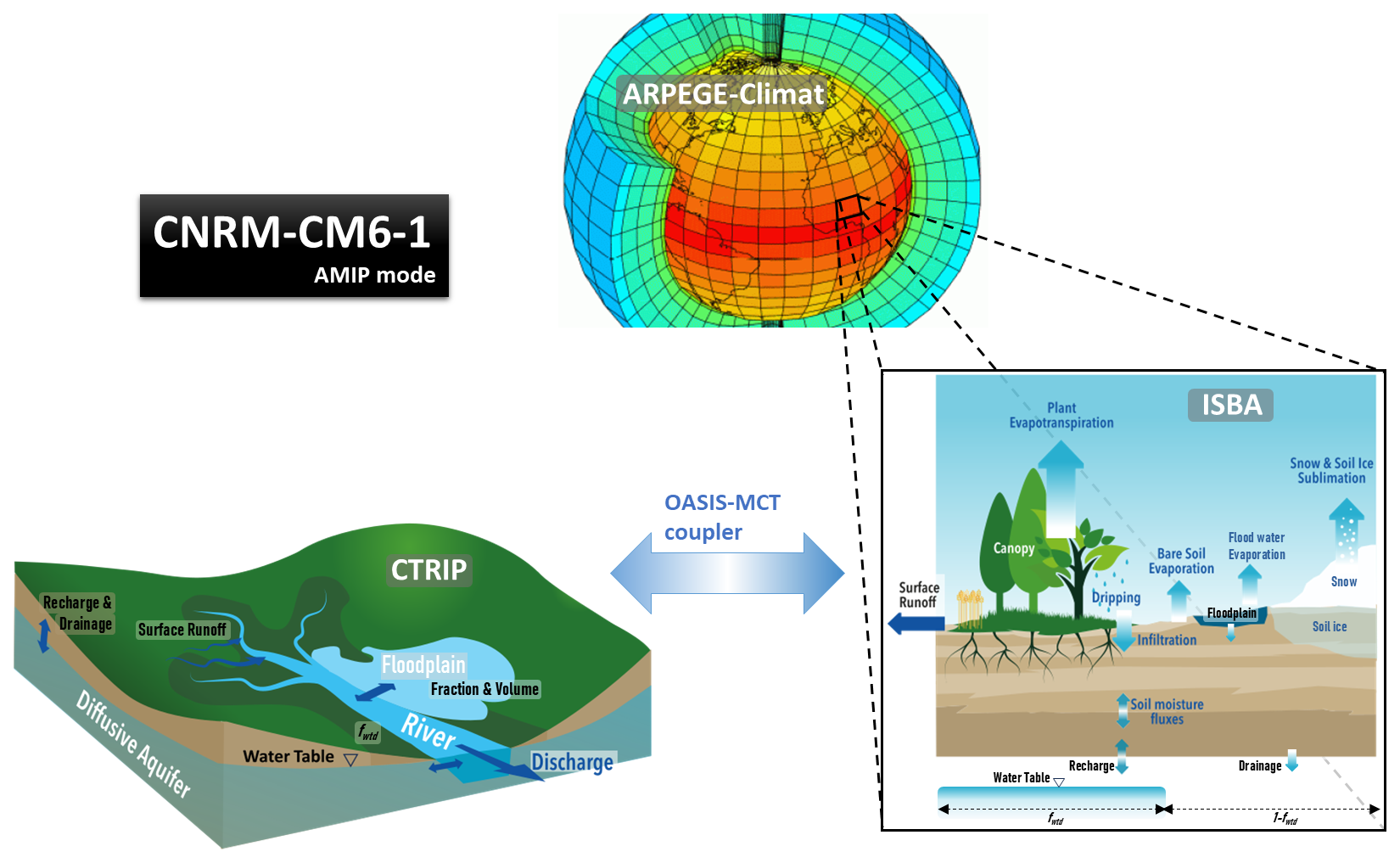
Figure 1 Schematic view of the CNRM-CM6-1 climate model in “AMIP mode”, which is not coupled to the NEMO ocean model. The model couples the ARPEGE-Climat v6.3 general circulation model with the ISBA-CTRIP system to simulate atmospheric, land surface, and hydrological processes. The ISBA land surface model includes a 1-layer vegetation interception scheme, CO₂-responsive plant transpiration, bare soil evaporation, snow sublimation, a 12-layer snow scheme, and a 14-layer explicit soil scheme for temperature, moisture, and soil ice. Soil moisture is computed within the rooting depth, which varies from 0.2 to 8 m depending on the vegetation type, while soil temperature is simulated down to 12 m. Subgrid hydrology accounts for surface runoff, deep drainage, and recharge fluxes, with groundwater interactions modeled over the low land fraction of the grid cell affected by the water table, f_wtd (illustrated by the gray footprint around the river). The CTRIP hydrological model simulates river discharge using total runoff from ISBA, dynamically solving river velocity with Manning's formula and incorporating a flooding scheme to compute flood volume and extent. It also includes a two-dimensional groundwater scheme for unconfined aquifers, representing time variations in water table depth, interacting with rivers and being fed by the recharge rate simulated by ISBA. The coupling between ISBA and CTRIP is achieved via the OASIS-MCT interface, allowing interactions between floodplains, soil, and atmosphere through evaporation, infiltration, and precipitation interception, as well as upward capillary fluxes into the unsaturated soil over f_wtd. Variables involved in these coupling processes are shown in black. Further details are available in Decharme et al. (2019).

2.1.2 The land surface

In CNRM-CM6-1, the land surface is represented by the ISBA-CTRIP land surface system, which is described in detail in Decharme et al. (2019) and only summarized here (Fig. 1). ISBA explicitly solves the one-dimensional Fourier and Darcy laws throughout the soil, accounting for the hydraulic and thermal properties of soil organic carbon. The soil moisture profile is computed within the rooting depth, which varies from 0.2 to 8 m depending on the vegetation type, as detailed in Fig. 2 and Table 1 of Decharme et al. (2019). These rooting depth values are derived from the ECOCLIMAP database. They reflect vegetation-specific adaptations to climatic and soil conditions. In contrast, the soil temperature profile is computed down to a depth of 12 m to account for thermal dynamics beyond the rooting zone. To represent land cover and rooting depth heterogeneities, a tile-based approach is employed. This approach allows multiple vegetation types to coexist within a single grid cell. Distinct energy and water budgets are computed for each tile, and their relative fractional coverage within the grid cell is used to determine the grid-box-averaged water and energy budgets. The use of a multilayer snow model of intermediate complexity allows separate water and energy budgets to be simulated for the soil and the snowpack. In the standard CNRM-CM6-1 model, the leaf area index (LAI) was prescribed from the ECOCLIMAP database. In our upgraded version, plant transpiration is controlled by the stomatal conductance of leaves, which depends on carbon cycling in vegetation; i.e., the LAI is prognostic and interacts with climate conditions as in the CNRM-ESM2-1 ESM (Delire et al., 2020; Séférian et al., 2019).

As regards the surface hydrology, a two-way coupling between ISBA and CTRIP is set up to account for (1) a dynamic river flooding scheme (Decharme et al., 2012) in which floodplains interact with the soil and the atmosphere through free-water evaporation, infiltration, and precipitation interception and (2) a groundwater scheme accounting for the world's 218 largest unconfined aquifer basins (Vergnes and Decharme, 2012; Vergnes et al., 2014) that combines two-dimensional diffusive groundwater flow between grid cells with vertical upward capillarity fluxes into the unsaturated soil allowed over a fraction of each grid cell, which varies with the elevation of the water table and its position with respect to the subgrid topography distribution (e.g., Fig. 2). The coupling between the aquifer simulated by CTRIP and the soil column simulated by ISBA has been modified compared to the standard version of the CNRM-CM6-1 climate model. While the standard coupling imposes the water table depth to be lower than or equal to the hydrological soil depth in ISBA to compute upward capillarity fluxes (Vergnes et al., 2014; Decharme et al., 2019), in our upgraded version, the Richards equation is modified to allow the water table to penetrate into the soil column of ISBA (Colin et al., 2023).

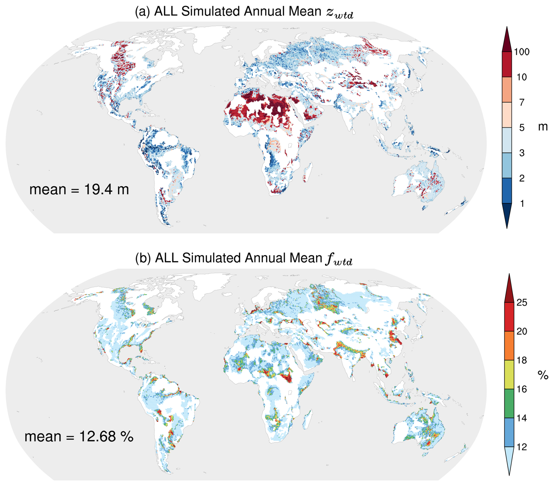
Figure 2 Groundwater behavior simulated by CNRM-CM6-1 (ALL experiment) during the 1980 to 2014 period at 0.5° resolution: (a) annual mean water table depth, z_wtd, and (b) annual mean subgrid fraction of the grid cell allowing vertical capillary rise, f_wtd, over the same period and at the same resolution. The global mean is given for each panel.

2.2 Experiments

We performed four experiments consisting of four ensembles of five simulations run over the 1980–2014 period with CNRM-CM6-1 driven by observed monthly SST and sea ice cover (SIC). The four experiments correspond to four configurations, noted as follows:

• ALL. The groundwater and floodplain schemes are both activated.

• CTL. The groundwater and floodplain schemes are both deactivated.

• GW. Only the groundwater scheme is activated.

• FLD. Only the floodplain scheme is activated.

For each experiment, a transient simulation was run over the 1850–1970 historical period, using restart files from a pre-industrial stabilized simulation run with the same configuration. The five members of each experiment were run over the 1970–2014 period, branching from the transient simulation – the ensembles are built using different restart files. The first 10 years are regarded as spinup. Results are analyzed over the 1980–2014 period. The various forcings used in CNRM-CM6-1 follow the CMIP6 recommendations (Eyring et al., 2016). SST and SIC are given by the Program for Climate Model Diagnosis and Intercomparison (PCMDI) AMIP Version 1.1.3 data set (Durack and Taylor, 2017). Greenhouse gas concentrations are prescribed from Meinshausen et al. (2017) using yearly global averages. The annual mean total solar irradiance forcing is given by Matthes et al. (2017). Many details on other forcings (i.e., tropospheric and stratospheric aerosols) are given in Roehrig et al. (2020).

2.3 Statistical significance computations

To assess field difference significance, we use the false detection rate (FDR) test from Wilks (2016), with a 95 % confidence level. It relies on t-tests performed for each grid point. However, instead of comparing the p values to a fixed value (0.05 for a 95 % confidence level) as is classically done, the FDR test consists of computing a threshold which also corresponds to a given confidence level (here 95 %) but depends on the series of all p values. This allows a reduction in the false detection rate (i.e., the detection of a signal which is actually not significant) in the case of auto-correlated fields, such as those analyzed in climate science. Further details on this test are given in Wilks (2016) and Colin et al. (2023).

3 Results

3.1 Groundwater levels and floodplains

In our model, groundwater processes are simulated over the world's 218 largest unconfined aquifer basins, giving access to the water table depth, z_wtd, over 43 % of the land surface (Fig. 2a). In the ALL experiment, z_wtd is shallower than 100 m over 40 % of the surface covered by the aquifers we represent, while more than one-third of this surface exhibits z_wtd between 1 and 10 m, which is coherent with the literature (Fan et al., 2013). On global average, z_wtd reaches a 19.4 m depth that is coherent with our estimates using offline simulations in a previous work (Decharme et al., 2019). Similar results are found in the GW experiment (not shown).

The temporal mean values of f_wtd, the fraction of each grid cell over which z_wtd is allowed to rise into the ISBA soil column (Fig. 2b), amount to 12 % of the area covered by the world's largest unconfined aquifer basins. In some regions known as the flattest in the world (the Niger delta, the Pantanal, the plains of the Ob basin, along the Amazon, the Ganges valley, the Netherlands, etc.), f_wtd can be significantly higher. Groundwater capillary flux to the above unsaturated soil only occurs in lowland near topographic depressions, rivers, or others water bodies (see Fan, 2015). In our groundwater scheme, these lowland fractions are computed in each grid cell using the actual distribution of the subgrid topography given by the Global Multi-resolution Terrain Elevation Data 2010 (GMTED2010; Danielson and Gesch, 2011) at a 7.5 arcsec (∼250 m) spatial resolution (see Vergnes et al., 2014; Decharme et al., 2019; and Colin et al., 2023, for more details).

The seasonal river overflow floodplains simulated by the ALL experiment represent a small fraction of the total land surface (Fig. 3a). Logically, these floodplains are located in the same lowland regions described previously. These inundations are generally at a maximum in spring and summer over mid- and high latitudes of the Northern Hemisphere (Fig. 3b), that is, after the snowmelt period. It can last between 1 and 3 months and even more along the main rivers (Fig. 3c). Over South America and monsoon regions (western Africa and southern Asia), floodplains are at a maximum after the rainy season and can also last between 1 and 3 months, but they can be larger along the main rivers or over Mesopotamia, the Pantanal, the Indus valley, and northern China. Note that this global view of floodplain behavior is coherent with satellite estimates (Prigent et al., 2007) and with previous offline studies (Decharme et al., 2008; Yamazaki et al., 2011; Decharme et al., 2012). Finally, the share of floodwater direct evaporation in total evapotranspiration is globally negligible but can be regionally significant (Fig. 3d).

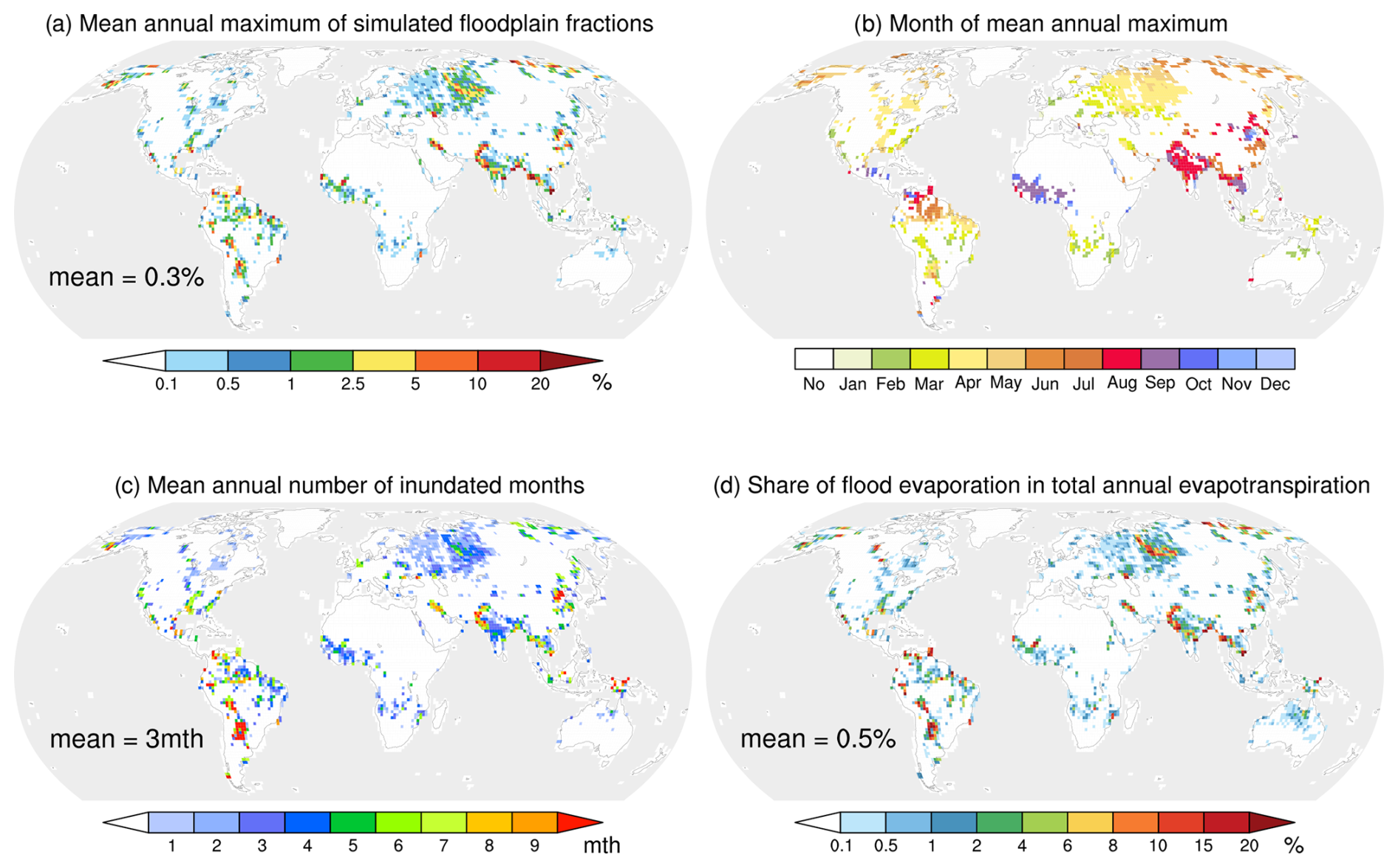
Figure 3 Floodplain behavior simulated by CNRM-CM6-1 (ALL experiment) over the 1980 to 2014 period: (a) maximum fraction of the mean annual cycle, (b) month where this annual maximum occurs, (c) number of months with a non-zero inundation fraction, and (d) share of floodwater direct evaporation in total annual evapotranspiration.

3.2 Land surface hydrological impacts

Time variations in terrestrial water storage (TWS) are very relevant to assess impacts of groundwater and floodplain processes on the simulated land surface hydrology at the global scale (Vergnes and Decharme, 2012; Decharme et al., 2019). Indeed, TWS is the sum of all hydrological reservoirs present at the Earth's surface, i.e., the water on the vegetation canopy, the snowpack, the inland water bodies, the soil moisture, and the groundwater. It is therefore the sum of all reservoirs simulated at the land surface by a climate model. The Gravity Recovery and Climate Experiment (GRACE) satellite mission, developed by NASA and the German Aerospace Center (DLR), measures temporal variations in the Earth's gravity field. These variations are used to estimate changes in terrestrial water storage (TWS), including surface water, soil moisture, and groundwater. Therefore, we used these GRACE data to evaluate the TWS variations simulated by our climate model (see also Data availability). This data set consists of an ensemble of three monthly TWS estimates from 2002 to 2014; they are derived from solutions provided by three independent processing centers: the Jet Propulsion Laboratory (JPL), the Helmholtz Centre for Geosciences (GFZ), and the Center for Space Research (CSR). These data are uniquely suited for evaluating large-scale hydrological processes, as they provide a global coverage of direct measurements which cannot be obtained through other observational products.

Figure 4 presents seasonal spatial patterns of TWS estimated by GRACE and simulated by the CTL and ALL experiments. For CTL and ALL, the spatial averages of bias and root-mean-square errors, compared to GRACE estimates, are also given. While the simulated patterns appear in good agreement with such estimates, ALL exhibits generally larger skill scores (mean bias and root-mean-square error) than CTL (except the bias from March to May (MAM) period), underlying the benefit of simulating groundwater and floodplain processes in a climate model to study land surface hydrology. This fact is confirmed in the seasonal cycles averaged over Siberia, North America, Amazonia, and southern Asia, where the ALL simulated cycles are closer than CTL to GRACE estimates. The GW and FLD experiments shown in the plots bring some interesting insights about the hydrological mechanisms involved. Over the tropics and sub-tropics, the improvement from CTL to ALL is mainly related to groundwater processes (GW seasonal cycles and square correlation closer than FLD to ALL). By storing the water during the rainy season to sustain river baseflow and surface soil moisture later during the dry season, groundwater processes increase the memory of the system and thus shift simulated seasonal TWS toward estimates. Over Siberia, and more generally over the north of the northern latitudes, improvements are generally attributable to the representation of river flood. During the snowmelt period, the river water overflows, and the resulting surplus is stored in large floodplains before it returns to the river later in the season. This buffer effect leads to a positive impact on the simulated seasonal TWS. Over northern mid-latitude regions, the impacts of flood and groundwater are equally distributed.

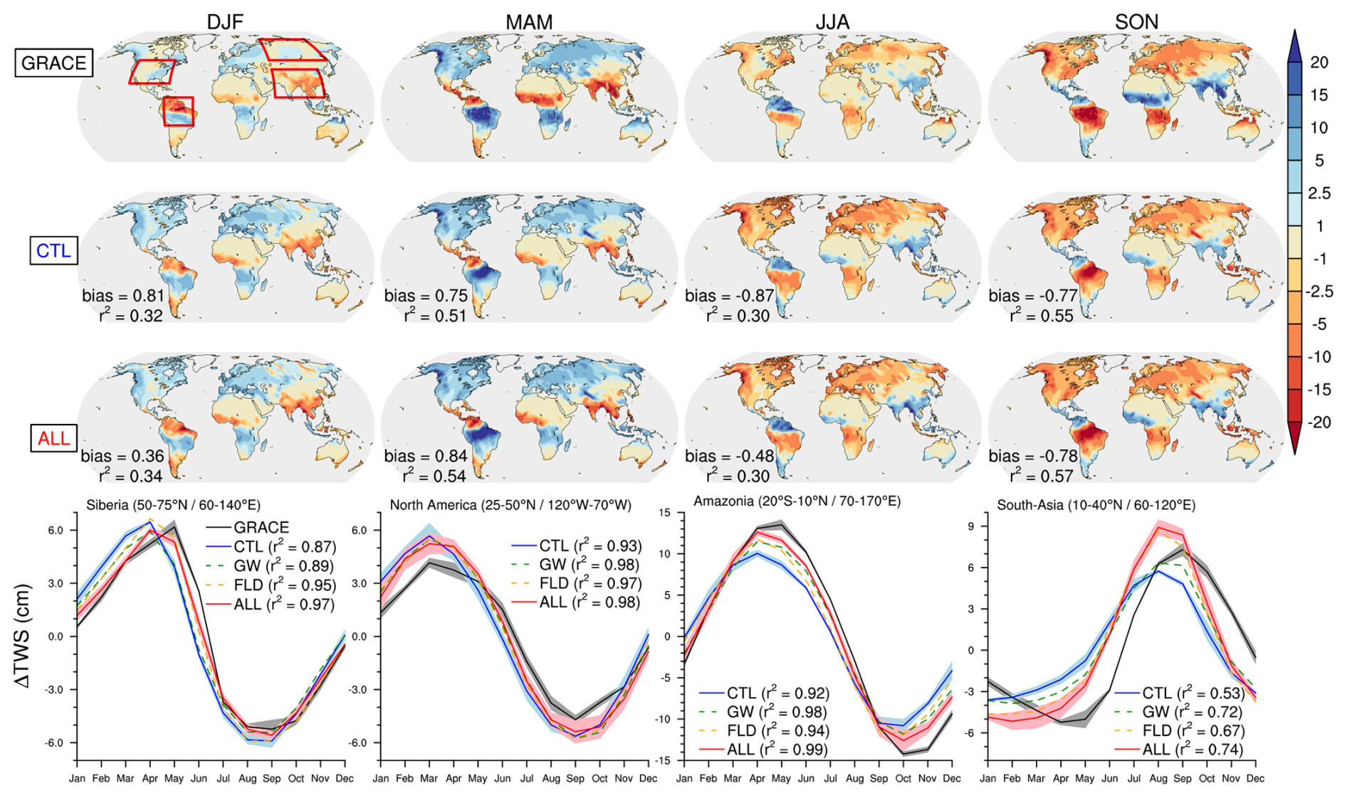
Figure 4 Estimated vs. simulated seasonal TWS variations (in cm) over the 2002 to 2014 period. Top panels show seasonal GRACE estimates and both the CTL and ALL simulated ensemble means. Global biases and patterns of squared correlations (r²) are given for each panel. Bottom plots show mean seasonal cycles averaged over four regions defined in red in the top-left panel. GRACE estimates are shown in black where shading corresponds to the minimum and maximum values of the ensemble of three GRACE solutions (JPL, GFZ, and CSR). Ensemble means of CTL in blue and ALL in red are given where shading shows ±1.64 times the intermember standard deviation, while ensemble means of GW (green) and FLD (orange) are shown with the dotted line. Square correlations (r²) between estimated and simulated mean seasonal cycles are given for each experiment.

River discharge is also a very relevant variable to assess the simulated water budget over large areas, whether using offline land surface models forced by atmospheric observations or coupled climate models. Beyond the direct evaluation of land surface hydrological processes, the comparison of simulated river discharges to observations allows the indirect evaluation of simulated precipitation over large basins. The climatological seasonal cycles of daily observed and simulated discharges near the mouths of the world's largest river basins are shown in Fig. 5 with the simulated vs. observed mean discharge ratio ($r_{\mathrm{d}}=Q_{\text{sim}}/Q_{\text{obs}}$) for the CTL and ALL experiments. Three subarctic basins (Mackenzie, Ob, and Lena), three temperate basins (Mississippi, Seine, and Danube), three tropical or sub-tropical basins (Amazon, Congo, Paraná), and three monsoon basins (Niger, Ganges, and Mekong) are represented. The simulated vs. observed mean precipitation ratio ($r_{\mathrm{p}}=P_{\text{sim}}/P_{\text{obs}}$) over each basin is also given for the CTL and ALL experiments. Details about river discharge observations are given in the Data availability section.

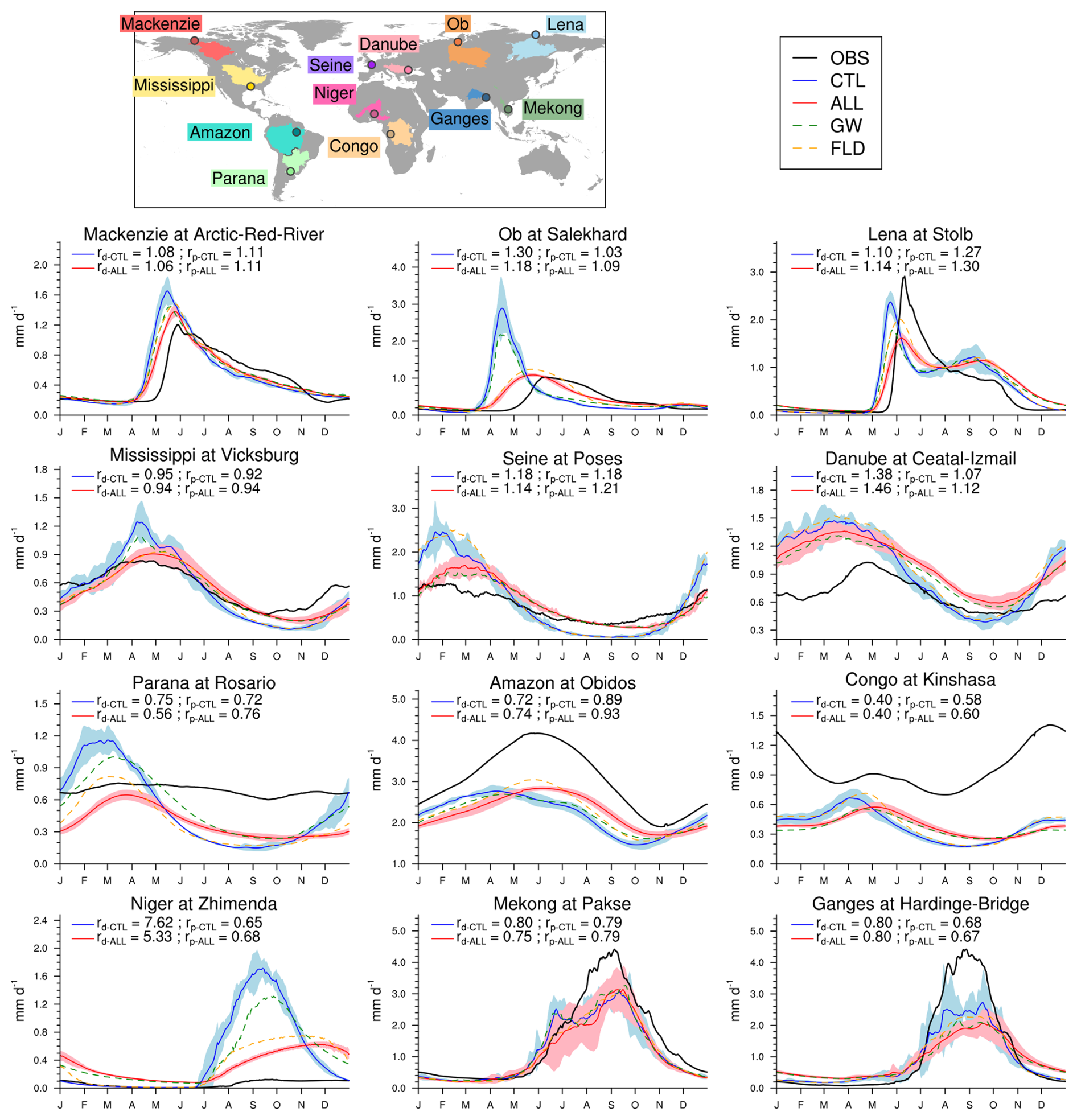
Figure 5 Comparison between the mean annual cycle (mm d⁻¹) of simulated and in situ measured daily river discharges near the outlet of the major basins of the world during the 1980–2010 period. Observations are in black, CTL is in blue, and ALL is in red, where shading shows ±1.64 times the intermember standard deviation. The annual simulated discharge ratio to observation (r_d) and the annual ratio of simulated to observed precipitation rates (r_p) are also shown for each basin and model. The observed precipitation rate used to calculate this ratio is the average of the same three products as in Fig. 11a. Additional GW and FLD experiments are also shown in green and orange, respectively, in each panel.

Over subarctic basins, ALL improves the simulated discharges compared to CTL, especially by reducing the lag and the intensity of the summertime peak of discharge. The simulated discharges remain, however, overestimated (r_d>1) in relation to the general overestimation of the simulated precipitation (r_p>1) over these basins. Regardless, the impacts of groundwater and especially floodplain processes are very positive over these regions. Additional GW and FLD experiments confirm that such improvement is mostly due to the floodplain processes. Mechanisms are relatively simple. The floodplain reservoir induces a buffer effect on river discharge by storing a large part of the springtime snowmelt runoff, thereby limiting the river streamflow velocity and thus the lag of the summertime peak of discharge. The reduction in this peak is explained by the direct evaporation of the water stored in the floodplains. This fact is especially noticeable over the Ob basin because of the high occurrence of floodplains (Fig. 3).

For temperate basins, the mean annual cycles for the observed river discharges are also better reproduced by ALL than by CTL. The main reason for these improvements is highlighted by the additional GW experiment (shaded green curves in Fig. 5). Aquifers store water during the rainy/snowmelt season, when the evapotranspiration is low, and thus contribute to delaying intense river discharges from the spring rainy/snowmelt season to the summer and/or autumn dry seasons (Vergnes et al., 2012; Vergnes and Decharme, 2012; Decharme et al., 2019). Over Europe, the river discharges are, however, drastically overestimated (see Seine and Danube), especially during winter and spring. This weakness is linked to the general overestimation of the simulated precipitation in these regions over this period (Fig. S1 in the Supplement). Conversely, summer precipitation is strongly underestimated, balancing the winter-to-spring overestimation and thus explaining why r_p is close to 1 over the Danube basin.

River discharge improvements are less obvious over tropical, sub-tropical, and monsoon regions due to a general underestimation of the simulated precipitation (Fig. 11a). In general, ALL simulated an annual peak of discharge later in the season than CTL. The resulting smoother mean annual cycles simulated by ALL seem to be more in phase (and thus in better accordance) with the observations than CTL. Over the Paraná, and to a lesser extent over the Amazon, the Mekong, and the Ganges, large floodplains (Fig. 3) contribute to a flattening of the annual peak of discharge due to the strong floodwater evaporation (Fig. 3d), while aquifers sustain baseflow during the dry season as over temperate basins. Over the Congo, aquifer processes are dominant partly because the strong underestimation of the simulated precipitation (r_p≪1) limits the development of floodplains. The case of the Niger is more special. While the ALL simulation appears in better agreement with observations, this agreement is not very convincing. As discussed in Decharme et al. (2019), the Niger basin has a very complex hydrodynamic structure with (1) many endorheic sub-basins in the north that do not contribute to the river flow due to a weakly connected drainage network and aridity, (2) the presence of deep aquifers that can be uncoupled from the river network, and (3) a large inner delta that favors an intensive evaporation loss and an important aquifer recharge leading to approximately 60 % of the inflow lost in the delta. About this last point, even if our model seems to be able to simulate a large inundation in the inner delta (Fig. 3a and d), this inner delta is not represented with enough detail to allow a realistic simulation of the Niger basin.

In conclusion, both the TWS variations and river discharges are generally improved by the addition of groundwater and floodplain processes in our climate model. The performance of coupled land–atmosphere models in reproducing the observed continental water masses and fluxes is closely related to the quality of the simulated precipitation. In the following subsection, we will see that groundwater and floodplains have a rather limited impact on the model's precipitation biases. So, as already highlighted in Decharme et al. (2019) using an offline setting of our land surface model, the improvement of the land hydrology with floodplains and groundwater is due to their capacity to increase the hydrological memory of the model while increasing the total evapotranspiration.

3.3 Climate impacts

We now focus on the impact of groundwater and floodplains on the simulated present-day mean climate (i.e atmospheric variables annually and seasonally averaged over the 1985–2014 period). As shown in the previous subsection, groundwater and floodplains act as continental reservoirs retaining water which would otherwise flow to the ocean, thus increasing TWS. The bulk of the increase in TWS with groundwater is located well below the root zone and therefore cannot be evaporated into the atmosphere. However, when the water table is shallow enough, the presence of groundwater leads to an increase in soil moisture in the root zone, through the combined effect of capillary rise and reduced drainage efficiency. Part of this additional soil moisture can be transported to the atmosphere through surface evaporation and plant transpiration. Floodplains constitute in themselves a reservoir of “evaporable” water, but the infiltration of water underneath floodplains also causes an increase in the root zone water content.

Figure 6 shows the mean annual increase in water stored in floodplains and in the root zone (Fig. 6a), along with the increase in evapotranspiration (Fig. 6b) in the FLD, GW, and ALL experiments, compared to the control experiment (CTL). The amount of evaporable water increases wherever floodplains are present and/or the water table is shallow. Results show that the presence of floodplains has a larger effect on evaporable water than that of groundwater (with a mean increase of 11.13 kg m⁻² in FLD and 6.59 kg m⁻² in GW). However, most of this increase in FLD and ALL is not due to the additional floodplain reservoir but to the increase in soil moisture in the root zone. In FLD (respectively ALL), water stored in floodplains accounts for 60 % (respectively 26 %) of the global increase in evaporable water, with an average spatial contribution of 30.7 % (respectively 20 %) (Fig. 7a). Water evaporated directly from floodplains represents an even smaller fraction of the increase in evapotranspiration (Fig. 7b), with a mean contribution of 17.4 % in FLD (10.3 % in ALL). Interestingly, the regions where this contribution is highest are generally not those where the increase in evapotranspiration is the largest (Figs. 5a and 6b). In other words, the increase in evapotranspiration in the presence of floodplains and groundwater is mostly due to a larger water content in the root zone.

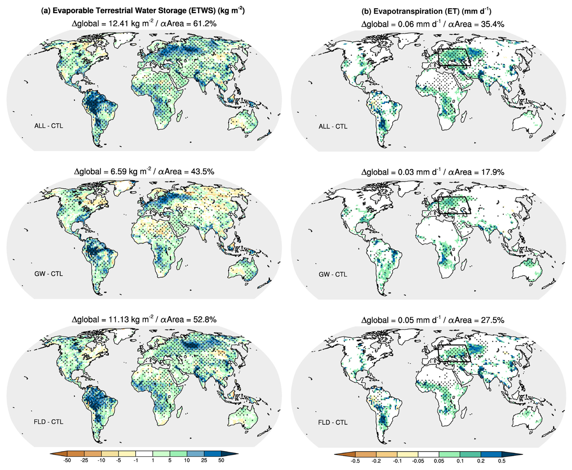
Figure 6 Impact of groundwater and floodplains on (a) evaporable terrestrial water (ETWS) (kg m⁻²), computed as the sum of the floodplain water storage and the root zone water content, and (b) evapotranspiration (ET) (mm d⁻¹).

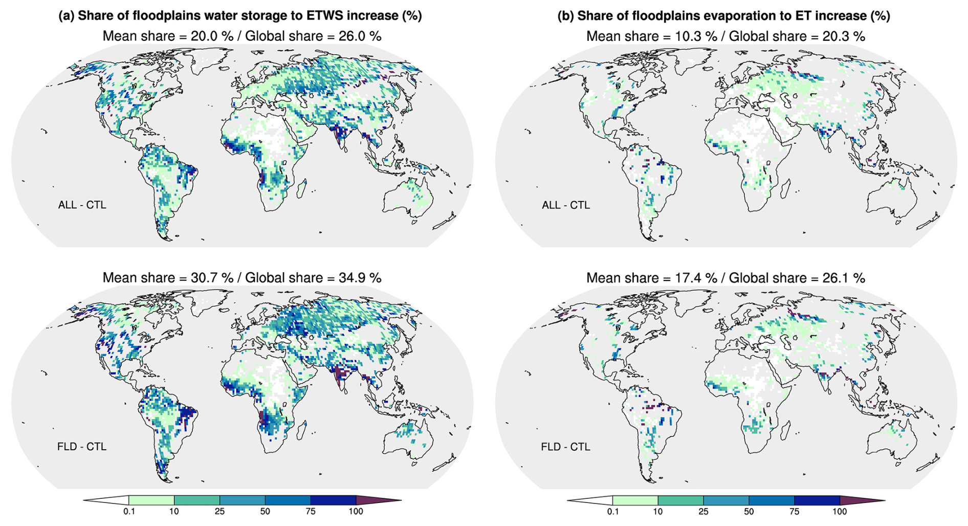
Figure 7 Contribution of floodplains to ETWS and ET. (a) Share of floodplain water storage to the evaporable terrestrial water storage (ETWS) shown in Fig. 6a. (b) Share of floodplain direct evaporation to evapotranspiration (ET) shown in Fig. 6b. The mean share corresponds to the spatial average of grid point shares. The global shares are computed as the contributions of the spatial sum of the floodplain variables (water content and evaporation) to the spatial sum of the reference variable (ETWS and ET).

As illustrated in Fig. 6b, the annual increase in root zone water content does not necessarily result in an increase in annual evapotranspiration. It is only when and where the evapotranspiration is limited by soil moisture, rather than by energy, that a larger amount of soil moisture (root zone water content) generates an increase in evapotranspiration Seneviratne et al. (2010). Groundwater can serve as an additional source of soil moisture in regions where evapotranspiration is limited by soil moisture, provided that the region exhibits a marked seasonality of precipitation. In such regions (generally characterized by high precipitation during the wet season), groundwater recharge can sustain a shallow water table during the dry season. This process is also applicable in areas of complex topography where groundwater converges in valleys (Fan, 2015; Colin et al., 2023). Similarly, the increase in soil moisture resulting from the infiltration of floodplain water can only lead to an increase in evapotranspiration in regions where the river discharge presents a pronounced seasonal cycle, linked with the precipitation seasonal cycle and/or the existence of a thawing season in the river catchment area.

To further explain the effects of groundwater and/or floodplains on the atmosphere, we focus on a region in eastern Europe where both groundwater and floodplains impact evapotranspiration (see box drawn in Fig. 6b). Figure 8 shows the seasonal cycles of the differences in liquid soil water content, evapotranspiration components, and air relative humidity, spatially averaged over this region, for each simulation with groundwater and/or floodplains (ALL, GW, FLD) compared to the control simulation (CTL) without groundwater or floodplains. The water content and relative air humidity differences are plotted along the vertical axis, representing soil depth and altitude, respectively. During the recharge season (November–April), the additional soil moisture in the GW simulation is located in the deeper layers of the soil column, which are closer to the water table depth or even beneath it. The upper layers are then either mostly frozen or already close to the field capacity in CTL. As the evaporative season progresses, the soil becomes drier, especially in the upper layers. Aquifers can then provide water to the unsaturated soil layers through capillary rise. Where the water table is shallow, the presence of groundwater also reduces drainage efficiency, resulting in a larger amount of soil moisture above the water table. This increase in soil moisture in GW leads to enhanced evapotranspiration, mostly through transpiration. With more soil moisture in the root zone, plants can transpire more water. Their growth is also enhanced (not shown), resulting in a further increase in the transpiration flux averaged over the region. The increase in leaf area also leads to a larger interception of precipitation by the vegetation, thus increasing the canopy evaporation. The soil moisture added with floodplains (FLD versus CTL) is expectedly larger in upper layers, as the additional water comes from the inundated surfaces above. It is visible from April–September in this region, where floodplains are present from December–July (see Fig. S2 in the Supplement). The floodplain evaporation is maximum in April, when the inundated surface is the largest (Fig. S2). As floodplains dry out, they give way to saturated surfaces, resulting in an increase in soil evaporation in FLD. As the warm season progresses, the vegetation grows and transpiration increases. In summer, the additional transpiration accounts for most of the increase in evapotranspiration in FLD, as it does in GW. The overall enhancement of evapotranspiration in GW and FLD results in a moistening of the lower troposphere, with an increase in relative humidity which can be seen from the surface up to approximately 2000 m. It is strong enough to foster a significant increase in summer precipitation (see Fig. S3 in the Supplement), which shows in annual precipitation (Fig. 10 for FLD). In return, the enhanced rainfall heightens the increase in soil moisture and evapotranspiration.

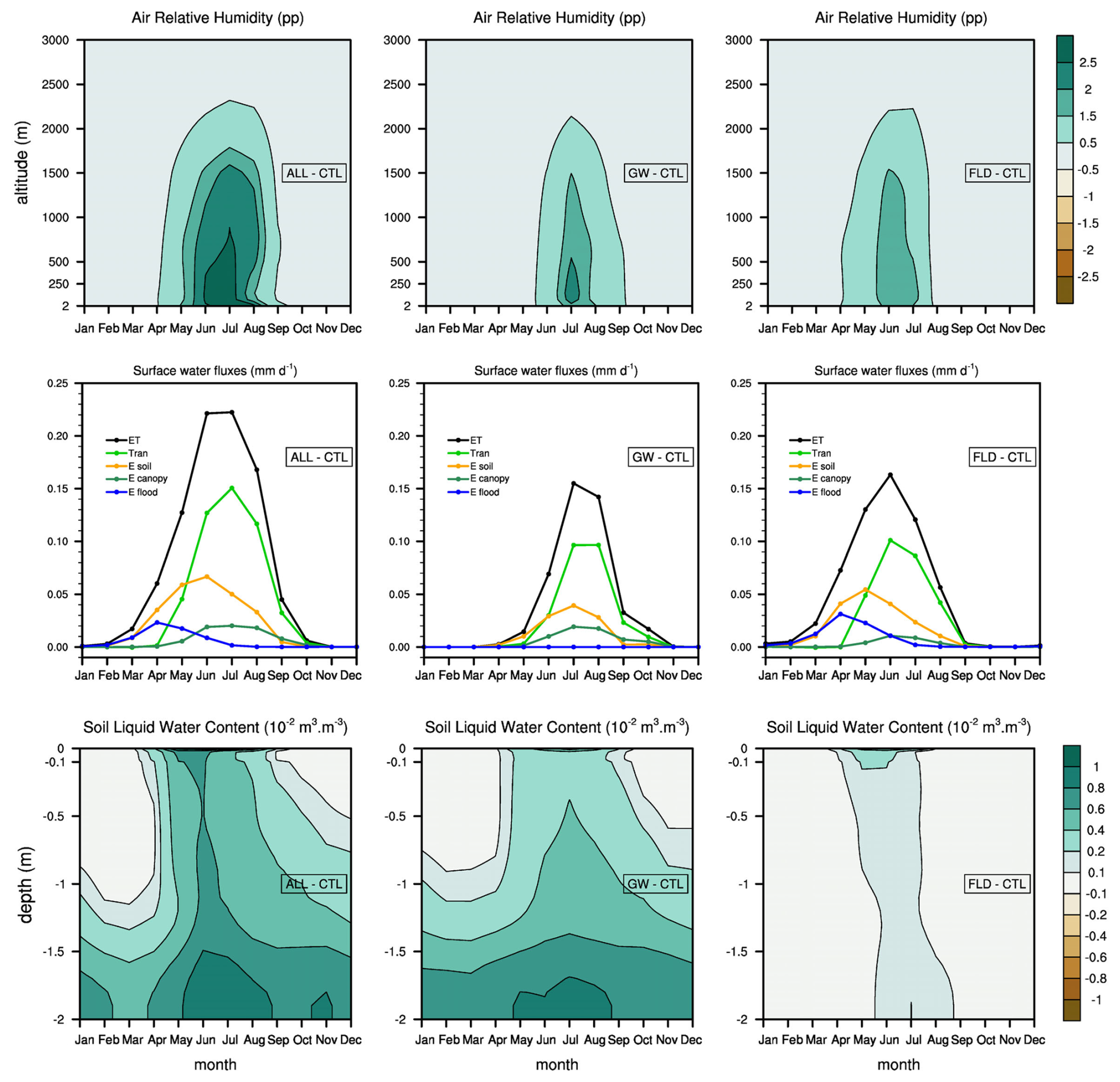
Figure 8 Mean seasonal cycle differences in relative humidity vertical profiles (percentage point; top), surface water fluxes (mm d⁻¹; middle), and soil liquid water content vertical profiles (10⁻² m³ m⁻³; bottom), spatially averaged over the “eastern Europe box” (40–60° N; 15–60° E). Left panels: ALL–CTL; middle panels: GW–CTL; right panels: FLD–CTL. The surface water fluxes considered are the total evapotranspiration (ET) and its components: transpiration (Tran), bare soil evaporation (E soil), evaporation of water intercepted by the canopy (E canopy), and floodplain evaporation (E flood). For each variable, statistically non-significant grid point differences are set to zero for the computation of the spatial average.

Over this particular region, the presence of groundwater has a stronger effect on soil moisture than that of floodplains. However, their respective impacts on evapotranspiration and air humidity have the same magnitude. This can be explained by the fact that floodplains affect the southern part of this region more (Fig. 6b), which is drier and thus more sensitive to the increase in soil moisture. The effects of groundwater and floodplains do not linearly add up in ALL, where both groundwater and floodplains are present. On average, over the region of Fig. 8, the water table is a little shallower in the presence of floodplains (see Fig. S2), as they increase the amount of water infiltrated into the soil. On the other hand, the floodplain surface is smaller in the presence of groundwater (see Fig. S2), as river–groundwater exchanges tend to dampen the river discharge seasonal cycle (see Fig. 5), thus reducing the maximum river height and the subsequent inundation. All in all, the combined effect of floodplains and groundwater on the hydrological variables depicted in Fig. 8 is less pronounced than the sum of the two individual effects.

Similarly to Fig. 8, Fig. 9 shows the seasonal cycles of the differences in soil temperature vertical profiles, surface heat fluxes (latent, sensible, and downward shortwave), and air temperature vertical profiles of ALL, FLD, and GW compared to CTL, spatially averaged over the same box as in Fig. 8. As could be expected, the soil temperature is cooler in the simulations with floodplains and/or groundwater (up to −0.5 °C). The heat capacity of water being greater than that of soil particles, a wetter soil is cooler (Al-Kayssi et al., 1990), hence the lesser soil temperature with the larger soil water content in ALL, FLD, and GW (see Fig. 8 during the summer season). This reduced soil temperature results in a decrease in the surface sensible heat flux, which is positive in this region during summer, that is, transporting heat from the surface to the atmosphere. This lessened heat transport in the presence of groundwater and/or floodplains contributes to a cooling of the atmosphere. However, the surface latent heat flux increase is stronger than the sensible heat flux decrease is. This means that the increase in evapotranspiration plays a bigger role in the atmosphere cooling (through a larger heat uptake) than the decrease in sensible heat flux does (through a lessened heat transport from the surface). With the increase in humidity in the atmosphere (see Fig. 8), there is also a reduction in the downward surface solar radiation, which also contributes to the cooling of the low atmosphere, but it is much smaller than the increase in latent heat flux. This shows that most of the decrease in the atmosphere temperature in GW, FLD, and ALL is due to the evapotranspiration increase in these simulations. In addition, given that this cooling occurs only in June and July, when the direct evaporation of floodplain water in FLD and ALL is negligible compared to the increase in bare soil evaporation and transpiration (Fig. 8), we can conclude that it is mainly driven by the evapotranspiration of the added soil moisture in the presence of groundwater and floodplains. This cooling of the atmosphere can be seen up to an altitude of approximately 2000 m.

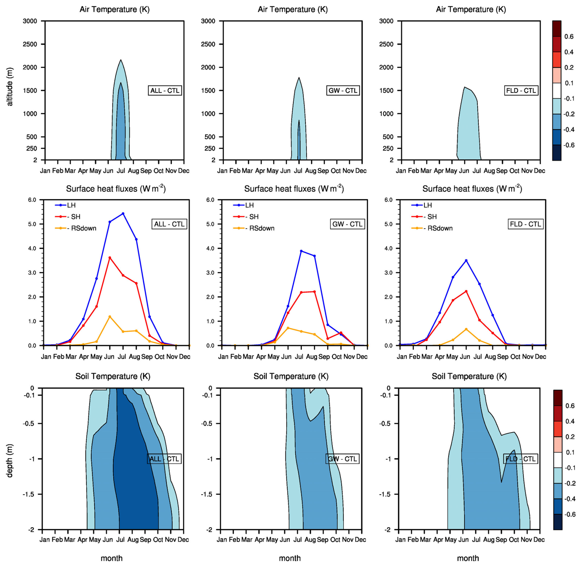
Figure 9 Mean seasonal cycle differences in air temperature profiles (K; top), surface heat fluxes (W m⁻²; middle), and soil temperature vertical profiles (K; bottom), spatially averaged over the “eastern Europe box” (40–60° N, 15–60° E). Left panels: ALL–CTL; middle panels: GW–CTL; right panels: FLD–CTL. The surface heat fluxes considered the turbulent latent (LH) and sensible (SH) heat fluxes and the downward solar radiation (RSdown). The latter two (SH and RSdown) are multiplied by −1. The spatial averages are computed as in Fig. 8.

Shifting back to a global perspective, we now consider the effect of groundwater and floodplains on the mean annual precipitation and 2 m air temperature worldwide (Fig. 10). Results indicate that floodplains have a larger impact than groundwater on both these variables, with a much greater percentage of the land surface affected by significant changes and larger mean differences. Focusing on precipitation changes, we find the presence of floodplains (FLD and ALL) leads to an increase in the mean annual rainfall in almost all of the regions of enhanced surface evapotranspiration (Fig. 6). This means that, in most cases, the increase in evapotranspiration over floodplain regions has enough effect on air humidity to result in larger amounts of precipitation. The situation is a little different when considering the addition of groundwater alone (GW). The presence of groundwater does not affect the annual precipitation anywhere, but it does lead to an increase in the mean summer (June–September) precipitation over the eastern European region (Fig. S3). Elsewhere, the increase in evapotranspiration induced by groundwater is not large enough and/or does not occur in the right season to affect precipitation. Conversely, the regions of increased precipitation are all affected by an increase in evapotranspiration, except for the central and northern parts of the Amazon basin, where the annual rainfall rate is larger in the presence of floodplains (ALL and FLD) without it being associated with an increase in the annual evapotranspiration – in fact, we find a decrease in evapotranspiration. Further analysis suggests that, over this region, humidity is transported from the floodplains of Venezuela, the mouth of the Amazon River, and/or northern Bolivia (not shown). The subsequent increase in annual precipitation leads to a larger mean cloud cover and a decreased downward solar radiation (see Fig. S4c in the Supplement). Since, over this humid region, evapotranspiration is limited by energy rather than by soil moisture, we find a decrease in evapotranspiration associated with the increase in precipitation. Everywhere else, the effects of groundwater and/or floodplains on precipitation remain circumscribed to the areas of evapotranspiration increase, meaning that the additional continental water induced by the presence of floodplains is transported only vertically in the atmosphere.

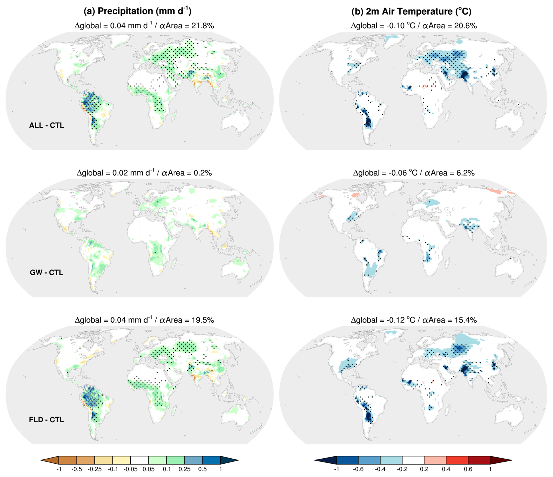
Figure 10 Impact of groundwater and floodplains on simulated annual mean (a) precipitation and (b) 2 m air temperature over the 1980–2014 period. Ensemble mean differences between CTL and ALL (first row), CTL and GW (middle row), and CTL and FLD (last row) are shown with their global values (Δglobal). The stippling indicates regions with statistically significant difference between CTL and ALL at a 95 % level of confidence using the FDR test. The percentage of the continental area (excluding Antarctica) which is statistically significant (αArea) is also given for each panel.

If we now consider the impact of groundwater and floodplains on 2 m temperatures (Fig. 10), we find a cooling of the near-surface atmosphere in most of the regions where the surface latent heat flux (i.e., evapotranspiration) is affected along with the surface sensible heat flux (see Fig. S4). Comparing the amplitudes of latent and sensible heat flux differences, we find that the increase in the former is larger than the decrease in the latter by a factor of 1.25 to 2 everywhere, except over a few grid cells in the eastern Sahara, where the differences are very small for both fluxes and the precipitation is barely affected. The downward surface solar radiation is also reduced with the presence of floodplains (FLD and ALL) in some of the regions of increased air humidity in the lower atmosphere (Fig. S4). However, the amplitude of this decrease in solar radiation remains limited (1 to 2 W m⁻²), and it mostly affects regions where the atmosphere cooling is not significant. In the few areas where the decrease in solar radiation is combined with a reduction in the 2 m temperature, we find that it is 1.5 to 3 times smaller than the increase in surface latent heat flux. Therefore, the decrease in 2 m temperature simulated in the presence of floodplains and/or groundwater is mostly due to evaporative cooling. This effect is stronger on warm temperatures, as the atmosphere evaporative demand increases with temperature. Indeed, we find a larger greater cooling of mean summer temperatures (compared to mean annual temperatures) and of mean daily maximum temperatures (compared to mean minimum temperatures), as shown in Fig. S5 in the Supplement for the boreal summer mean values.

Over some regions, the cooling of the lower atmosphere in the presence of floodplains (FLD and ALL) is associated with a slight increase in the sea level pressure mostly in the Northern Hemisphere during the boreal summer (see Fig. S6 in the Supplement). However, this effect on pressure quickly fades with the altitude, as there is no significant impact of groundwater or floodplains on the geopotential heights above the 925 Pa level (not shown). We also found no significant impacts on the mean values of wind components, regardless of the altitude (not shown). Thus, groundwater and floodplains have no significant impact on the atmosphere dynamics in our simulations, at least from a climatic perspective (that is, on annual and seasonal averages over a fairly long period). As mentioned before, their effects on the atmosphere's temperature, humidity, and precipitation remain “local” almost everywhere, in the sense they occur above land surfaces affected by an increase in evapotranspiration. In other words, there is no significant advection of the temperature and humidity changes, except in central and southern Amazonia, where the additional air humidity is transported from floodplains located in regions nearby. To sum up, representing groundwater and floodplains in our model leads to an increase in precipitation and a cooling of warm temperatures in a number of regions worldwide, with a larger impact from floodplains. Whether or not these impacts improve the model's biases is addressed in the following paragraphs. This last piece of our analysis does not include a thorough discussion on the bias sources, as this has already been done in Roehrig et al. (2020).

The model's annual precipitation biases are shown in Fig. 11a for the CTL and ALL experiments (details about precipitation observations are given in the Data availability section). As already pointed out (Sect. 3.2), whatever the experiment, a drastic underestimation of precipitation is found over the tropics. Elsewhere, the amplitude of the annual bias is much more acceptable. However, these biases can vary greatly depending on the season (Fig. S1). For example, over central Eurasia or the US Great Plains, winter precipitation is generally overestimated, while summer precipitation is underestimated. Comparing the CTL and ALL biases in regions where the differences between CTL and ALL are statistically significant (Fig. 11a), we find that groundwater and floodplains reduce the underestimation of precipitation in Africa, South America, and central Eurasia. This amounts to a mean global improvement in precipitation and to a larger land surface area impacted by an improvement than by a worsening of the bias. In central Eurasia, the bias reduction is due to the increase in summer precipitation (June–September), which can be attributed mostly to groundwater in the western part of the region and to floodplains in the eastern part (see Figs. S1 and S3). In South America, the increase in precipitation is almost entirely due to floodplains and occurs during the austral summer (December–March) (Figs. S1 and S3). In Africa, the improvement is again due to floodplains, and it occurs during the rainy season, which corresponds to the boreal summer above the Equator (Figs. S1 and S3) and spans from October–February in southern Africa (not shown).

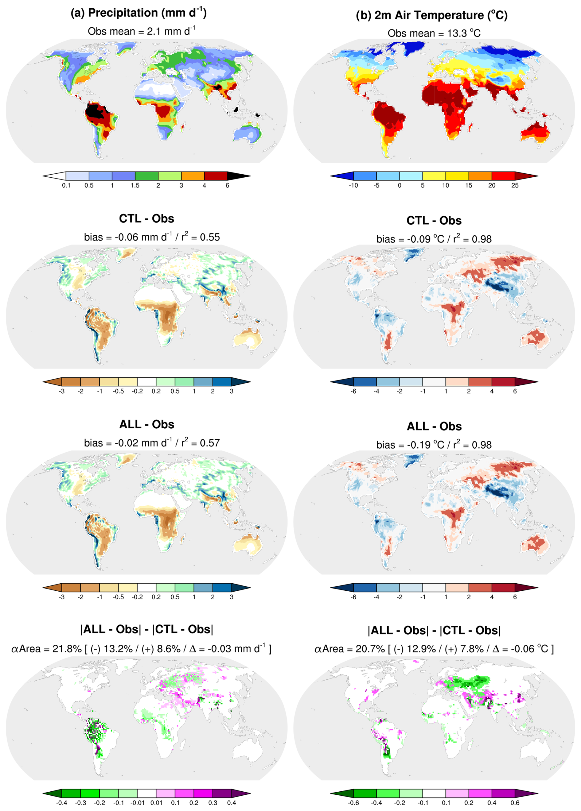
Figure 11 Observed vs. simulated annual mean (a) precipitation and (b) 2 m air temperature over the 1980–2014 period. The first row shows observations and their global mean values. The middle row shows both the CTL and the ALL ensemble mean biases compared to observations with their global biases and patterns of squared correlations (r²). The last row shows differences between these CTL and ALL absolute biases over regions with statistically significant differences between CTL and ALL at a 95 % level of confidence using the FDR test (see Sect. 2.3). A negative value (green) means an improvement (i.e., ALL closer to observations than CTL), and a positive value (purple) means a deterioration. The percentage of the continental area (excluding Antarctica) where this difference is statistically significant (αArea), the global mean of this difference (Δ) over this area, and the percentage of the continental area with negative (−) and positive (+) values are also given.

The annual biases of 2 m air temperatures are shown in Fig. 11b for the CTL and ALL experiments (see Data availability for details on observations). A warm bias is found over the Pantanal region, central and southern Africa, eastern Siberia, central Eurasia, and Australia, while Greenland and the Himalayas show a cold bias. In the Northern Hemisphere, the cold biases occur in winter and the warm ones are seen mainly in summer, except for eastern Siberia, which shows a warm bias in winter (Fig. S7 in the Supplement). In the Pantanal region and Australia, the warm bias persists throughout the year, with a larger amplitude during the austral summer (December–March). In central Africa, the warm bias is stronger during the austral winter (June–September), and, in southern Africa, the warm bias is only seen during this season (Fig. S7). As is the case for precipitation, the impact of groundwater and floodplains on the 2 m air temperature biases is mostly positive. It consists of a reduction in the warm biases found in the Pantanal throughout the year and in central Eurasia in summer (Fig. S7). In the Pantanal, the improvement is almost entirely due to floodplains. In central Eurasia, the cooling induced by the presence of groundwater reduces the bias over the western part of the region, while floodplains cool the eastern part (Fig. 10). During the boreal summer, the combined effects of floodplains and groundwater also reduce the warm bias over parts of the US (Figs. S5 and S7).

As previously explained, the decrease in air temperature and increase in precipitation induced by floodplains and groundwater is mostly due to the additional evapotranspiration and air humidity. In the regions where this leads to a reduction in the temperature and precipitation biases, we find that the model's evapotranspiration and air humidity are mostly underestimated in the CTL experiment and that this dry bias is improved in ALL (Fig. 12 and Figs. S8 and S9 in the Supplement). Therefore, the impact of groundwater and floodplains on the model's biases of temperature and precipitation biases does not result from a compensation of errors. The representation of groundwater and floodplains does really improve our model's realism by adding missing processes.

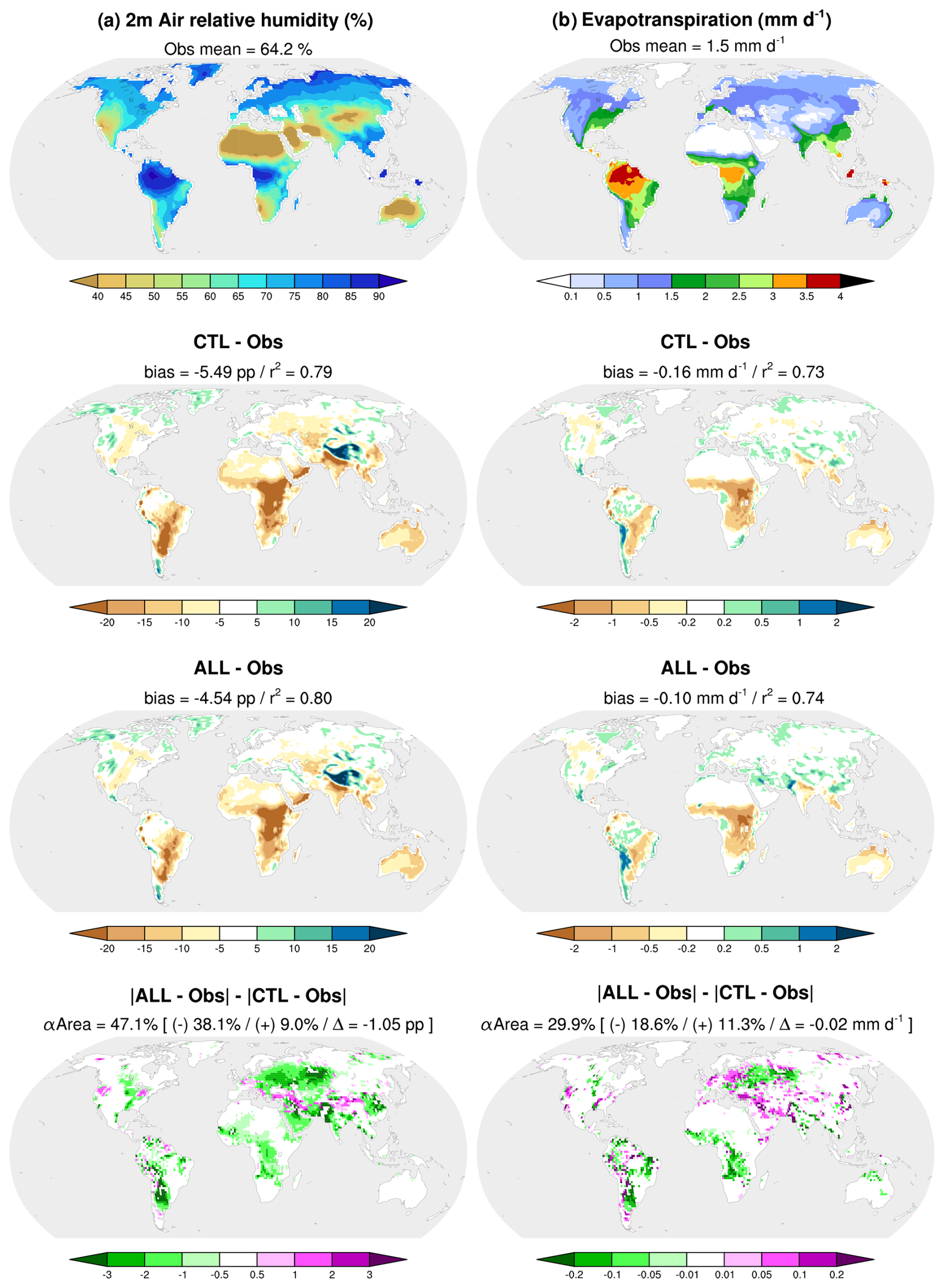
Figure 12 Observed vs. simulated annual mean (a) 2 m air relative humidity over the 1980–2014 period and (b) land surface evapotranspiration over the 1982–2008 period. The first row shows observations and their global mean values. Notations are the same as in Fig. 11. Relative humidity differences are given in percentage points (pp).

4 Discussion and conclusions

The inclusion of floodplain and groundwater processes in the CNRM climate model has demonstrated significant improvements in the simulation of land surface hydrology and climate in a number of regions. One of the primary impacts on land hydrology is the enhanced accuracy in terrestrial water storage variations and river discharges. This improvement is attributed to the increased hydrological memory and surface evapotranspiration brought about by the integration of groundwater and floodplain dynamics. As already highlighted in Decharme et al. (2019), using an offline setting of our land surface model, the extended hydrological memory allows the model to better represent the seasonal variability in water storage and flows, leading to more accurate simulations of river discharge and terrestrial water storage. Despite these positive outcomes, the model reveals several notable discrepancies when compared to observed river discharge data. These deficiencies can be attributed to simulated precipitation biases in certain regions, but they can also be attributed to model weaknesses. For example, the Niger basin is poorly simulated, which is likely due to a lack of representation of its highly complex hydrodynamic structure. In regions of the world where these issues are prevalent, basin-by-basin work will be essential in the future to advance the representation of hydrological processes in our climate model.

Regarding climate variables, the inclusion of these processes has led to increased surface evapotranspiration and in regions where this flux is primarily driven by soil moisture. This results in a decrease in near-surface air temperatures, particularly warm ones, and an increase in precipitation in those areas, effectively reducing the impact of the model's biases on these variables. Importantly, these improvements are not the result of error compensation. They are based on more realistic representation of land–atmosphere interaction as evidenced by the comparison of simulated evapotranspiration and air humidity with observational data, showing that biases in these variables are also reduced with the inclusion of groundwater and floodplains. The processes involved here are consistent with previous studies showing that inland water bodies can influence the atmosphere by humidifying and cooling its lower layers throughout an increase in evapotranspiration (Bonan, 1995; Lofgren et al., 2002; Krinner, 2003; Balsamo et al., 2012; Le Moigne et al., 2016; Arboleda Obando et al., 2022).

It is, however, important to note that the overall changes induced by floodplains and groundwater on atmospheric climate variables remain relatively small when compared to the existing biases. This suggests that, while these processes significantly enhance the model's hydrological components, their impact on climate variables is more modest. Nonetheless, the improvements in land hydrology processes are significant, which in itself justifies the inclusion of these processes in global climate models. Moreover, incorporating these processes in a coupled model framework allows the representation of feedback mechanisms between the land surface and the atmosphere. These feedbacks are essential for understanding the complex interactions that drive climate dynamics. By capturing these interactions, the model can provide more comprehensive insights into the hydrological and climatic processes, thereby improving the overall quality of climate simulations.

In addition to the water cycle, incorporating these processes in ESMs is important to study the impact of climate and hydrology on the carbon cycle and vice versa. Soil moisture is a key driver of natural CO₂ emissions, regulating both plant behavior and the microorganisms that decompose organic matter in the soil (Canadell et al., 2021; Friedlingstein et al., 2023). However, the impact of groundwater on soil decomposition and carbon emissions remains largely unexplored to date, even though it acts as lower boundary conditions for soil moisture. Using groundwater schemes in ESMs could help fill this gap. The use of the floodplain scheme in ESMs is also important for understanding the interplay between hydrology and methane emissions, especially at the inter-annual timescale. Floodplains, with their dynamic water levels and saturated soils, are ecosystems poor in oxygen. These anaerobic conditions favor methane production from the decomposition of soil organic matter (Saunois et al., 2020; Morel et al., 2019). Hence, simulating the distribution and variations of such surface water bodies over the global land surface in ESMs is also a key question regarding climate change and projection of greenhouse gas emissions.

Finally, anthropogenic processes, such as irrigation and dams that can alter the river flow and increase the continental evapotranspiration (Sacks et al., 2009), are not accounted for in our model. Looking ahead, our next step is to incorporate these anthropogenic water fluxes into the model (Druel et al., 2022; Sadki et al., 2023; Decharme et al., 2025). This addition aims to further enhance the representation of land hydrology and its interactions with climate. By doing so, we hope to achieve an even more accurate and comprehensive simulation of the coupled land–atmosphere system, ultimately contributing to better predictions and understanding of future climate scenarios.