Potential for equation discovery with AI in the climate sciences

Climate change and artificial intelligence (AI) are increasingly linked sciences, with AI already showing capability in identifying early precursors to extreme weather events. There are many AI methods, and a selection of the most appropriate maximizes additional understanding extractable for any dataset. However, most AI algorithms are statistically based, so even with careful splitting between data for training and testing, they arguably remain emulators. Emulators may make unreliable predictions when driven by out-of-sample forcing, of which climate change is an example, requiring understanding responses to atmospheric greenhouse gas (GHG) concentrations potentially much higher than for the present or recent past. The emerging AI technique of “equation discovery” also does not automatically guarantee good performance for new forcing regimes. However, equations rather than statistical emulators guide better system understanding, as more interpretable variables and parameters may yield informed judgements as to whether models are trusted under extrapolation. Furthermore, for many climate system attributes, descriptive equations are not yet fully available or may be unreliable, hindering the important development of Earth system models (ESMs), which remain the main tool for projecting environmental change as GHGs rise. Here, we argue for AI-driven equation discovery in climate research, given that its outputs are more amenable to linking to processes. As the foundation of ESMs is the numerical discretization of equations that describe climate components, equation discovery from datasets provides a format capable of direct inclusion into such models where system component representation is poor. We present three illustrative examples of how AI-led equation discovery may help generate new equations related to atmospheric convection, parameter derivation for existing equations of the terrestrial carbon cycle, and (additional to ESM improvement) the creation of simplified models of large-scale oceanic features to assess tipping point risks.

1 Introduction

Addressing climate change caused by fossil fuel burning presents a three-fold challenge to society and science. The first is to determine what constitutes a broad “safe” maximum level of global warming, for which there are already proposals of 1.5 or 2.0 °C (UNFCCC, 2015) above preindustrial times. One guide is to constrain global warming to levels that avoid triggering large-scale tipping points (TPs) (e.g. Abrams et al., 2023) (or even a self-perpetuating cascade of TPs; Wunderling et al., 2021), where major changes would occur to Earth system components for relatively small additional temperature increases. The second challenge, once a warming threshold is adopted, is supporting adaptation planning by determining detailed local changes in near-surface meteorology corresponding to that global temperature rise. Third is deriving greenhouse gas (GHG) emissions profiles compatible with the stabilization of global warming at prescribed target levels. Knowledge of such profiles may encourage mitigation plans to develop non-fossil-fuel energy sources sufficiently fast to prevent key global warming threshold exceedance. All three challenges depend on an accurate knowledge and simulation of the global coupled climate–carbon cycle system in response to fossil fuel burning. The reports of the Intergovernmental Panel on Climate Change (IPCC), of which the latest is the sixth assessment (IPCC, 2021), present the current state of such understanding, while also highlighting the substantial remaining uncertainties in key climate components. Such uncertainties aggregate, preventing the constraining of summary global parameters such as equilibrium climate sensitivity (ECS), which is global warming in a stabilized climate for doubling of atmospheric CO₂ concentration. The range of ECS values estimated by Earth system models (ESMs) remains substantial (Forster et al., 2021). Also, for many regions, there remains large uncertainty in how hourly to annual rainfall levels will change as GHGs rise (e.g. Tebaldi et al., 2021), including for extremes (Lenderink et al., 2017; Lenderink and Fowler, 2017). Uncertainty in ECS leads to poor knowledge of CO₂ emissions reductions compatible with keeping global warming below a target such as 2 °C. Uncertainty in future changes to rainfall statistics prevents adaptation planning for any altered future flood or drought frequencies.

ESMs are complex computer codes designed to estimate climate change for prescribed trajectories of potential future atmospheric GHG concentrations or emissions. The basis of ESMs is the numerical discretization (at scales of typically 100 km) of equations that describe all Earth system features, including the oceans, land surface, atmosphere, and cryosphere, and their feedbacks. Analysis of ESM diagnostics has enabled breakthroughs in climate system understanding, and a community achievement is that approximately 20 research centres contribute model output to a common database available for evaluation by researchers. The latest ensemble of models is the Coupled Model Intercomparison Project version 6 (Eyring et al., 2016). However, the large uncertainties (as noted above) are derived from differences between ESMs. Hence, a key requirement for climate researchers is understanding and removing such differences to create refined projections with smaller uncertainty bounds. An interim approach to uncertainty reduction is the method of emergent constraints (e.g. Hall et al., 2019; Williamson et al., 2021; Huntingford et al., 2023), which searches for inter-ESM regressions between simulated quantities that are also measured and changes in importance in the future. Measurements use any robust identified regressions to constrain bounds on future quantities. However, while emergent constraints provide a powerful methodology to lower inter-ESM spread, ultimately all ESMs need improved equation representation yielding more accurate simulations.

As climate science has progressed through ESM development in recent decades, so have artificial intelligence (AI) algorithms. The potential applications of AI in society are vast, including opportunities to advance scientific discovery (e.g. Wang et al., 2023). As expected, there are calls to apply AI to climate science (Jones, 2017) and in detail (e.g. Schneider et al., 2017; Huntingford et al., 2019; Reichstein et al., 2019; Eyring et al., 2024). Already AI has been found to have a strong ability to warn about emerging extreme climate events (e.g. Bi et al., 2023; Lam et al., 2023) and the timing or onset of key oscillatory features of the climate system, such as the Madden–Julian oscillation (MJO) (Delaunay and Christensen, 2022). Yet most AI algorithms are statistically based, creating interest in applying newer physics-informed methods (Karniadakis et al., 2021) to support understanding climate components (Kashinath et al., 2021). Physics-informed approaches strive to retain at least some consistency with known underlying process differential equations. Examples of applications include the reconstruction of atmospheric properties of tropical cyclone events (Eusebi et al., 2024) and characteristics of extreme precipitation (Kodra et al., 2020).

Even more recently, a branch of AI has emerged termed “AI-led equation discovery” which derives candidates for the governing equations that describe any dataset under investigation. Unlike physics-led approaches, the technique instead uses AI to discover hereto unknown equations, with the method proposed by Raissi et al. (2019, their Sect. 4) and Champion et al. (2019), Brunton et al. (2016), and Rudy et al. (2017). As described above, the advancement of ESMs implies the development of the equations encoded in them. Hence, we consider how this AI technique may support ESMs by discovering any required missing equations and parameters.

2 AI methods and including for equation discovery

2.1 Background climate analysis methods and existing AI methods

The range of AI methods is vast. Selecting the correct one depends on data attributes such as frequency, spatial size, and extent of system non-linearity. If there are “labels” describing the effects searched for, this suggests using supervised rather than unsupervised algorithms. Advances in the knowledge of geophysical processes and related mathematical models have traditionally driven the development of ESMs. However, climate research has also been influenced by statistically based approaches and methods, some of which are precursors to more modern AI techniques. In this section we (1) review some traditional statistical approaches to climate analysis; (2) describe the application of generic and currently available AI algorithms to climate science; (3) review currently available AI algorithms in a general non-climate context; and (4) consider newer techniques, including physics-informed calculations, again for the broader application background. To achieve this summary and for all four points, we point to and make summaries of four influential textbooks (Fig. 1). We select “keywords” from some section headings of Storch and Zwiers (1999) for an initial statistical analysis of climate attributes. Early applications of machine learning applied to environmental issues, including forecasting and components of the climate system, are presented in Hsieh (2009). For a general but extensive overview of available machine learning algorithms, we use Murphy (2013). Moving more towards the central theme of this perspective, Brunton and Kutz (2022) summarize very current methods of data-driven machine learning, including physics-led techniques.

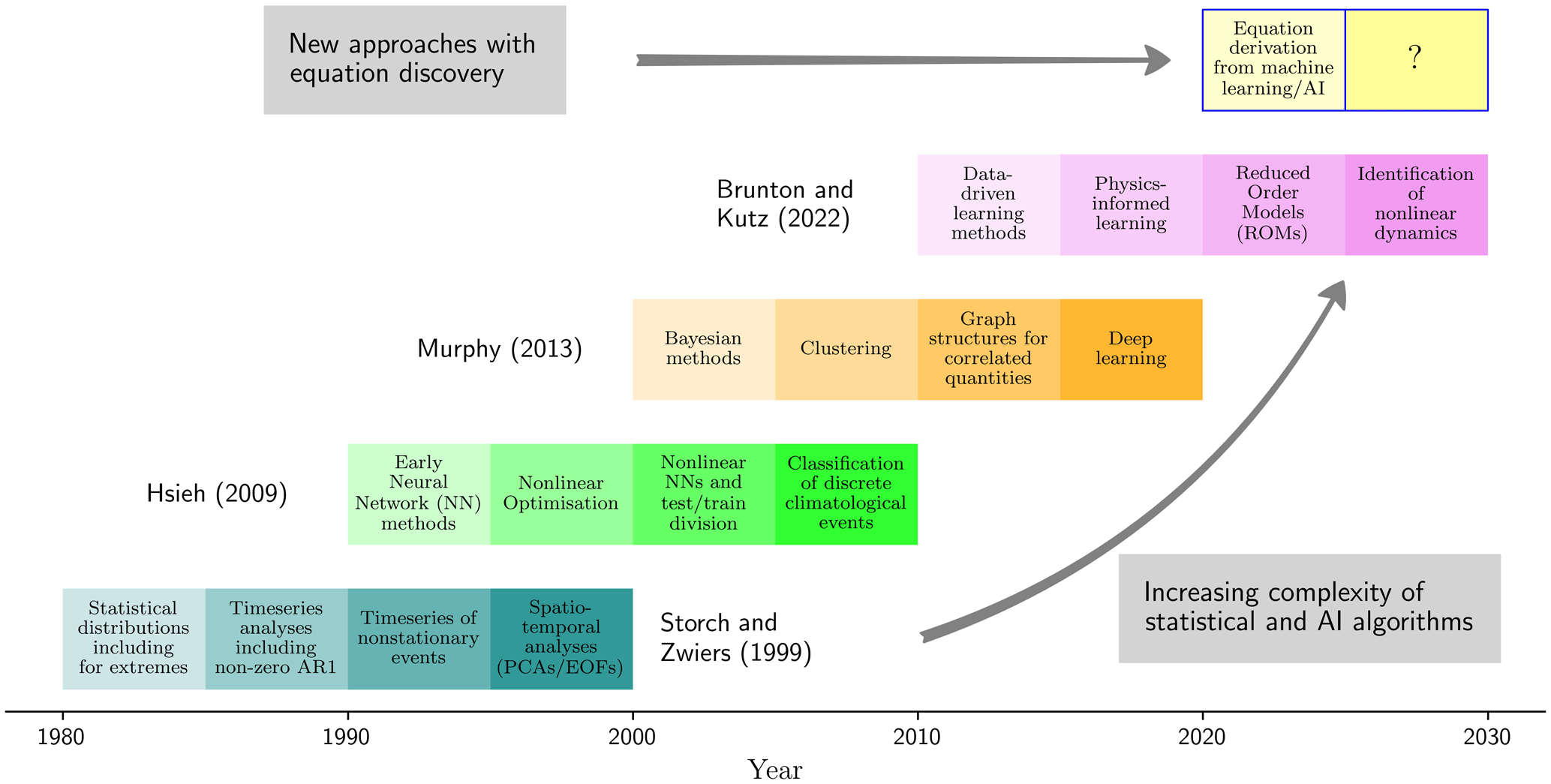
Figure 1 Schematic illustrating the evolution of the application of statistical methods to climate research, as well as more recent general developments in AI methods. The techniques illustrated and applied to environmental research are based on sections of the books by Storch and Zwiers (1999) and Hsieh (2009). More generic AI developments, not necessarily used in climate research, are linked to parts of the books by Murphy (2013) and Brunton and Kutz (2022), where the latter describes newer physics-led algorithms. The top bar suggests using recent advances in AI that are capable of deriving underlying process equations to determine better features of the climate system where uncertainty remains. The call for applying AI-led equation discovery to climate research is the main subject of this commentary. We retain the idea that AI may also support climate research in ways not yet considered, as shown by the question mark.

In more detail, Storch and Zwiers (1999) describe the initial application of statistical methods to climate-related research, including probability theory, time series analysis, Eigen techniques, and empirical orthogonal functions (EOFs). The EOF method is popular for spatio-temporal analyses of physical climate variables (Smith et al., 1996; Mu et al., 2004; Hannachi et al., 2007). EOFs reduce the degrees of freedom of key variables (such as sea surface temperatures; Smith et al., 1996), often presented as spatial patterns capturing geographical modes of variability multiplied by time series of their magnitudes. EOFs enable a simpler way to characterize climate models and therefore allow easier comparison against gridded datasets (e.g. Mu et al., 2004). Inspired by how the human brain is believed to operate, early neural networks evolved from the perceptron model to hidden-layer models (Hsieh, 2009). Standard multivariate regression and EOF methods contain strong implicit assumptions of linearity, while neural networks in all forms contain non-linear elements. Also of importance is the widespread application of Bayesian statistics in climate science. Bayesian statistics provide information on state variables, including a priori knowledge about such quantities, and therefore hint at the newer physics-led approaches. The application of deriving Bayesian probability distributions for climate quantities matured during the first decade of the 21st century. For example, Berliner et al. (2000) employ such methods to detect and attribute human forcing of the climate system, as represented by near-surface temperature fields. Boulanger et al. (2006) determine the dominant features of the temperature variability in South American data, which is then used to compare to the performance of the ESMs at generating such variations and from this weight such models and hence their future projections. Similar Bayesian-based analyses for near-surface temperature but for multiple regions across the globe are performed by Smith et al. (2009).

Most early studies with AI inputs focus on supervised learning, where model training uses a subset of labelled target data, and the remaining data are used to test predictive performance. However, in recent decades, clustering algorithms have substantially increased the popularity of unsupervised learning. Unsupervised learning, by definition, raises the exciting possibility of algorithms that interpret climate data or ESM-based outputs in new ways. The broad analysis of Steinbach et al. (2003) uses clustering to identify climate indices that characterize many behaviours of the oceans and the atmosphere. Similarly, Lund and Li (2009) use clustering of autocorrelated climate time series to identify the areal limits of distinct climate zones. Graphical models, also an unsupervised method, provide a novel technique to find links between variables of interest. Ebert-Uphoff and Deng (2012) use such models to explore causal relationships between atmospheric circulations and provide a framework with much potential to discover further relationships between climate variables.

Many scientific problems, including climate research, involve the interpretation of exceptionally large datasets. The advent of “big data” methods has enabled the analysis of climate models and data to generate better forecasting methods, supporting earlier or enhanced warnings of extreme events. For example, Liu et al. (2008) assessed different data-driven learning methods to downscale weather forecasts to provide statistics of near-surface meteorological conditions at single points or very small spatial scales and to include predictions of local extremes. Additionally, the climate system contains strong and complex non-linear interactions that operate over multiple timescales, including forecasting. Yet, despite this complexity, robust underlying reduced-complexity non-linear dynamical system descriptions may await discovery. Traditional scale analysis of underlying equations can reveal such dynamical systems, which led to the famous paper of Lorenz (1963), providing a three-variable system of coupled ordinary differential equations (ODEs) that simulate aspects of atmospheric convection. One suggestion is that newer algorithms may routinely identify the dominant processes in complex systems, such as the long short-term memory (LSTM) technique (a recurrent neural network algorithm; Vlachas et al., 2018), designed to forecast high-dimensional chaotic systems. Recent studies also highlight deep learning methods that analyse key datasets to improve medium-range weather forecasting (Bi et al., 2023; Lam et al., 2023). Although these two examples are for much shorter timescales than emerging climatic signals on decade-to-century timescales, they illustrate the usefulness of AI in extracting additional information from complex atmospheric data.

Reduced order models (ROMs) project the dominant processes described by partial differential equations (PDEs) onto low-rank spaces. The method improves the computational speed and optimization of any fully parameterized PDE system. As such, ROMs enable behaviours of the full PDE model to be better evaluated and understood more quickly. Proper orthogonal decomposition (POD) is a key method for creating a ROM, used to study complex spatio-temporally dynamic systems in fluid dynamics (e.g. for oceanic circulations; San and Iliescu, 2015), and provides a viable way to interpret ESM diagnostics. EOFs are an earlier form and a subset of ROMs. We suggest that the full utility of ROMs and their many potential configurations and applications are largely unexplored for climate science. Brunton and Kutz (2022) make a case for deriving a process interpretation for the main components of any ROM-type decomposition.

Despite remarkable progress, most AI methods are statistical in construction. There is a growing view (again reflecting the Bayesian viewpoint) that AI needs to recognize there are often underlying processes for which substantial knowledge exists. Hence, physics-informed learning is gaining traction, providing methods of constraining machine-learning-based predictions using physical laws. Karniadakis et al. (2021) reviewed embedding physics in machine learning and concluded that combined data and physics-based model integration is achievable even in uncertain and high-dimensional contexts. That research discussed several applications of physics-informed learning for inverse and ill-posed problems in fluid dynamics, thermodynamics, and seismology, illustrating the possibility of increased process consistency but expressed via neural network architectures.

We now turn to a new frontier in AI development, which we suggest is of potential extensive use in climate science. In this next step, where uncertainty exists in the underlying physical processes, AI derives the underlying descriptive equations. Such discoveries can constitute either a full equation set or a smaller reduced-complexity set that captures the dominant system responses. The upper row of Fig. 1 presents this as an emerging direction for machine learning (ML) or AI (we use the terminology of ML and AI interchangeably; see Kuehl et al., 2022, for precise definitions and how the two differ).

Equation discovery using ML is well positioned to advance our understanding of Earth's climate, which contains non-linear features, given that the basis of much AI is to find underlying non-linearities. A specific approach is symbolic regression, the most common AI-based approach to discovering equations implicit in data. This form of regression procedure searches a space of mathematical expressions to find the optimal combination (i.e. a symbolic model) that best fits the data. Sparse regression is a symbolic regression method with the advantage of diminishing the search space of possible terms in the equation discovery process, substantially reducing the likelihood of over-fitting to observed data. Brunton and Kutz (2022) place a special emphasis on a sparse regression method, sparse identification of non-linear dynamics (SINDy), a data-driven approach to uncover ROMs of systems with unknown spatial-temporal dynamics.

2.2 Symbolic regression methods for equation discovery to uncover unknown dynamics

Equation discovery techniques can be categorized as data-driven or knowledge-driven discovery (Tanevski et al., 2020). These approaches involve inferring the best possible derived model structure and parameter values by ensuring minimal error between observations and model predictions. The former approach, considered to be general AI-led equation discovery, is applicable for systems where there is very little or no understanding of the underlying dynamics and, therefore, no obvious model structure pre-exists. The latter approach relies on existing expert knowledge of the system, in which those developing the discovery process ensure features of the existing models remain in the new derived equations.

A field of AI already existing is that of explainable AI (Linardatos et al., 2021). This approach defines a set of methods and techniques that provide accessible and understandable justifications for predictions with ML, which are often “black-box” models such as neural networks. However, we make an important distinction that AI-led equation discovery can be considered more useful, instead as a form of interpretable AI, due to its inherent ability to produce human-readable and interpretable mathematical expressions as outputs. By default, the equations themselves are generally explainable. However, in some cases where the generated equations are complex and unintuitive, explainable AI methods may be needed to make the expressions more comprehensible (Aldeia and De França, 2021).

Where the behaviours of a dynamical system are largely or completely unknown, an emerging method to determine the underlying equations is that of symbolic regression. The data-driven symbolic regression algorithm does not depend on user-specified prior knowledge of a system. Hence, unlike a usual regression task that involves a predefined model structure, symbolic regression finds the optimal model and its parameters that best fit the data.

The usual form of symbolic regression, which can effectively minimize both model complexity and prediction error, is sparse regression, which is the main focus of this section. However, we first note other methods, such as a deep-learning-based symbolic regression model proposed by Petersen et al. (2019) that uses a recurrent neural network with a “risk-seeking policy gradient” to generate better fitting expressions. This approach has been shown to be robust against noisy data.

Deep neural networks have the inherent capability to approximate non-linear functions, and, in certain set-ups, can also accurately approximate non-linear operators. For instance, the DeepONet model developed by Lu et al. (2021) can approximate a diverse range of non-linear continuous operators from data such as integrals, as well as implicit operators that represent deterministic and stochastic differential equations. We briefly mention an issue that can arise with AI methods, known as the “closed-world assumption” (Chen and Liu, 2018). This issue arises if not all relevant knowledge is contained within the available data forming the training dataset. This may lead to a situation where previously unseen dynamics not captured during an AI training period may be present in the data held for testing and is therefore not recognized by the model. AI models operating with this assumption cannot update themselves with new information especially in open and dynamic environments, where new features in data continually appear. We also note a novel data-driven method for solving ODEs and PDEs rather than “discovering” them, as introduced by Cao et al. (2023). In Cao et al. (2023), the Laplace neural operator is utilized for solving differential equations that can account for non-periodic signals, unlike the more well-known Fourier neural operator. The Laplace neural operator is an alternative approach to the more traditional numerical solvers and can be advantageous since it has the capability to rapidly approximate solutions over a wide range of parameter values and without the need for further training.

Another type of symbolic regression method is that of genetic algorithms (GAs) (Keren et al., 2023). GAs can include prior physical knowledge of the system in the optimization procedure, and they work particularly well for systems with strong linearity. This technique involves building “trees” of random symbolic expressions and using stochastic optimization to perform the replacement and recombination of tree subsamples. Ultimately, this finds the combination of terms that best fit the data.

Common to these three symbolic regression methods (sparse regression, deep learning, and GAs) is an optimization procedure which finds a linear combination of (potentially non-linear) functions from a large functional space which best fits the underlying system behaviour. The quickest and most general approach is to use sparse regression, which substantially reduces the search space of possible functions. Such speed is needed, compared to a computationally inefficient “brute-force” method of looping over all combinations of possible contributing functions. Sparse regression also reduces the likelihood of over-fitting, generating equations with limited terms, although sufficient to explain the features of the underlying datasets. A popular sparse regression algorithm developed by Brunton et al. (2016), known as sparse identification of non-linear dynamics (SINDy), identifies the simplest (parsimonious) model that describes the dynamics of non-linear systems implicit in data. SINDy investigates time series data to extract interpretable and generalizable models in the form of ordinary differential equations evolving in time. In the event of multiple time series spanning a spatial region, SINDy can then determine partial differential equations. A general dynamical system model takes the form of $\dot{\mathit{x}}\left(t\right)=\mathit{f}\left(\mathit{x}\right(t\left)\right)$, where the vector $\mathit{x}=\begin{array}{cccc}\left[x_{\mathrm{1}}\right(t)& x_{\mathrm{2}}\left(t\right)& \cdot \cdot \cdot & x_d\left(t\right){]}^{\mathrm{T}}\in {\mathbb{R}}^d\end{array}$ represents the state of the system at a single time instance, t, consisting of d system variables. The SINDy algorithm finds a function $\mathit{f}:{\mathbb{R}}^d\to {\mathbb{R}}^d$ defining the dynamics and time evolution of the system. Collecting a time history of the state $\dot{\mathit{x}}\left(t\right)$ across the m set of times $t_{\mathrm{1}},t_{\mathrm{2}},\mathrm{\dots },t_m$ produces the complete m×d data matrix.

$$\begin{array}{}\text{(1)}& \mathbf{X}=\left[\begin{array}{c}{\mathit{x}}^{\mathrm{T}}\left(t_{\mathrm{1}}\right)\\ {\mathit{x}}^{\mathrm{T}}\left(t_{\mathrm{2}}\right)\\ \mathrm{⋮}\\ {\mathit{x}}^{\mathrm{T}}\left(t_m\right)\end{array}\right]=\left[\begin{array}{cccc}{x}_{\mathrm{1}}\left(t_{\mathrm{1}}\right)& x_{\mathrm{2}}\left(t_{\mathrm{1}}\right)& \mathrm{\cdots }& x_d\left(t_{\mathrm{1}}\right)\\ x_{\mathrm{1}}\left(t_{\mathrm{2}}\right)& x_{\mathrm{2}}\left(t_{\mathrm{2}}\right)& \mathrm{\cdots }& x_d\left(t_{\mathrm{2}}\right)\\ \mathrm{⋮}& \mathrm{⋮}& \mathrm{\ddots }& \mathrm{⋮}\\ x_{\mathrm{1}}\left(t_m\right)& x_{\mathrm{2}}\left(t_m\right)& \mathrm{\cdots }& x_d\left(t_m\right)\end{array}\right]\end{array}$$

The symbolic regression task is to find the form of f from a time series of the state X(t) that maps to the derivative $\dot{\mathbf{X}}\left(t\right)$ and that is valid across the m set of times $t_{\mathrm{1}},t_{\mathrm{2}},\mathrm{\dots },t_m$ at which data are available. In order to find a sparse representation of f, an augmented library, we first start with Θ(X), consisting of n candidate functions. The individual functions contributing to f may include polynomial and trigonometric terms. This construction gives a library of dimensions $n\times m\times d$. We show this construction below, where the horizontal direction (size n) are the candidate functions, the vertical direction (size m) are the time steps, and “out of the page” is size d, which are the different state variables. In the matrix Θ(X) below, functions can include “cross terms”, so for instance a quadratic term X² and for d=2 would have $x_{\mathrm{1}}^{\mathrm{2}},x_{\mathrm{2}}^{\mathrm{2}}$ and additionally x₁x₂ terms (see Eq. 2 of Brunton et al., 2016).

$$\begin{array}{}\text{(2)}& \mathbf{\Theta }\left(\mathbf{X}\right)=\left[\begin{array}{ccccccccc}|& |& |& |& & |& |& |& |\\ \mathbf{1}& \mathbf{X}& {\mathbf{X}}^{\text{2}}& {\mathbf{X}}^{\text{3}}& \cdot \cdot \cdot & \sin \mathbf{X}& \cos \mathbf{X}& \sin \mathrm{2}\mathbf{X}& \cos \mathrm{2}\mathbf{X}& \cdot \cdot \cdot \\ |& |& |& |& & |& |& |& |\end{array}\right]\end{array}$$

The sparse regression problem is then set up as $\dot{\mathbf{X}}\left(t\right)=\mathbf{\Theta }\left(\mathbf{X}\right)\mathbf{\Xi }$, where we want to solve for the matrix Ξ∈ℝ^nd, which contains vectors of n coefficients corresponding to the linear expansion for each of the d state variables, $\mathbf{\Xi }=\left[\begin{array}{llll}{\mathit{\xi }}_{\mathrm{1}}& {\mathit{\xi }}_{\mathrm{2}}& \mathrm{\cdots }& {\mathit{\xi }}_d\end{array}\right]$. For simplicity, looking at this regression problem for only one system variable, let y be a vector of data measurements (i.e. a column of X), where y∈ℝ^m. The fitting procedure is then attempting to minimize the difference between y and Θξ since y=Θξ, where Θ(X)∈ℝ^mn and ξ∈ℝⁿ. In the case of multiple variables, this becomes a multi-regression problem as previously introduced, and the minimization is a single sweep across all state variables and so is not the best fit for each individual variable.

Various sparse regression optimizers can solve for ξ. A common algorithm known as LASSO introduces sparsity to the regression procedure via an L¹ regularization term: $\mathit{\xi }=\underset{{\mathit{\xi }}^{\prime }}{\mathrm{argmin}}{∥\mathbf{\Theta }{\mathit{\xi }}^{\prime }-\mathit{y}∥}_{\mathrm{2}}+\mathit{\lambda }{∥{\mathit{\xi }}^{\prime }∥}_{\mathrm{1}}$. The key result of solving for Ξ using sparse regression is that the coefficient vectors that it obtains are sparse (where most entries are set to zero) due to the optimization procedure. This means that only a few non-linear terms in the candidate library are active and therefore included in the right-hand side of one of the row equations ${\dot{\mathit{x}}}_k={\mathit{f}}_k\left(\mathit{x}\right)$. This leads to a sparse representation of f and therefore parsimonious dynamical models.

A particularly comprehensive verification of the capability of sparse identification to derive equations is presented in Chen et al. (2021). In that analysis, and pretending to have no knowledge beforehand of the underlying equations, five fundamental governing equations are reproduced purely from data. These equations are those of Burgers, Kuramoto–Sivashinsky, non-linear Schrödinger, Navier–Stokes, and a reaction–diffusion equation. Although we place an emphasis in this section on sparse regression for equation discovery where we might have little or no knowledge of underlying model structures beforehand, this method may also be used where there exists some process understanding. Such an application is closer to a physics-informed approach. In these circumstances, the library Θ is restricted to take only a limited set of functional forms based on such a priori knowledge, possibly allowing faster convergence of the optimization procedure as some components of the dynamical system are known.

The SINDy algorithm can additionally include forcing variables in the sparse representation of the dynamics, known as “SINDy with control” (Brunton et al., 2016). This configuration gives the ability to simultaneously disambiguate the internal dynamics of a system and the effect of forcing variables. For climate modelling, an external forcing variable could be a time series of GHG emissions, their atmospheric concentration levels, or radiative forcing that integrates the effect of all changes in different GHG concentrations. One of the important properties of dynamical systems is stability, which is not guaranteed with the standard SINDy regression algorithm. For physical systems involving fluid flows where the underlying equations are known to be energy-preserving, although also non-linear (e.g. having quadratic terms), the “trapping SINDy” algorithm is available, based on the Schlegel–Noack trapping theorem (Kaptanoglu et al., 2021). This algorithm offers necessary conditions for the discovered models to be globally stable and energy conserving. We note that the confirmation of basic conservation properties is a cornerstone of ESM development and testing. The SINDy algorithm was originally used to only discover systems of ODEs but was quickly extended to search for PDEs, using an algorithm known as “PDEFIND”, which fully captures the spatial-temporal behaviour of dynamical systems (Rudy et al., 2017).

There are computer packages that implement the SINDy algorithm and its configurations (for example, trapping capability), for ODE and PDE systems, such as the Python-based PySINDy package (Brunton et al., 2016).

3 Potential applications of AI-led equation discovery

We discuss the potential application of AI-led equation discovery to three Earth system components. In each example, there is presently a deficiency in understanding, causing uncertainty in the representation of processes by equations and their parameterization. Each application falls into one of three categories.

In the first example, we address the requirement to better parameterize small-scale convective events at the larger scale to enable their planet-wide representation in coarser-scale Earth system models. In this instance, arguably, we do not understand the form of the governing equations valid at larger scales.

In the second example, we consider closing the global carbon cycle, where the largest uncertainty is often the magnitude of atmosphere–land CO₂ exchanges. We suggest seeking parameters valid at the large ESM gridbox scale, although initially for placement in existing land equations. Due to parameter uncertainties, global land–atmosphere CO₂ exchange is often derived as a residual, after contemporary CO₂ emissions and changes in atmospheric and oceanic carbon content are accounted for (e.g. Canadell et al., 2007), circumnavigating using a land surface model. However, while this provides valuable contemporary information, it prevents predictions of future land changes. Land surface models are improving (Blyth et al., 2021) with new key processes already represented by equations, but their parameterization may apply only at the field scale or smaller, depending on data used for calibration. Yet the land surface is heterogeneous, providing an opportunity for algorithms to determine equation parameters that instead aggregate fine-scale processes to ESM gridbox scale. In some other instances, terrestrial processes do remain poorly understood, and so equation discovery may also identify additional equation terms that capture such effects. Hence we focus on whether AI may advance existing equations by deriving parameters valid at large spatial scales but note that discovery methods might also characterize missing processes in equation form.

Our third example concerns ocean circulations where the governing equations are fully understood at the local scale, but of interest is how their internal interactions aggregate to create regional and global responses. Spatially upscaled computationally fast equations can generate key knowledge of oceanic response for a broad range of potential future GHG trajectories that ESMs have not simulated. Many reduced-complexity large-scale ocean models exist, but the equations are presently estimates. We conjecture that AI-generated spatial aggregation may refine such equations. An additional benefit is that comparing these simpler models with large-scale oceanic measurement datasets may provide summary information on the performance of ESMs from which AI has derived the large-scale equations.

3.1 Large-scale parameterization of fine-resolution convective events

The representation of convection remains a major shortcoming in traditional ESMs, where grid scales of 50–200 km cannot explicitly resolve convection, necessitating parameterization. These empirical parameterizations simulate sub-grid vertical displacement of mass, energy, and water on the ESM gridbox scale, producing modelled rainfall. However, common convective parameterizations often fail to capture typical diurnal cycles of cloud cover and rainfall (Fosser et al., 2015; Prein et al., 2013), with rainfall estimates that are too frequent and light. Such parameterizations also struggle to represent long-lived convection that propagates across multiple gridboxes, organizing the atmosphere on the mesoscale (Stephens et al., 2010). Meanwhile, rainfall intensities are rising with global temperatures, scaling with the water-holding capacity of a warmer atmosphere at 7 % K⁻¹ on average, following the Clausius–Clapeyron relationship (e.g. Westra et al., 2014). However, this statistic does not account for complex meso-scale dynamics unresolved by ESMs. Thus, shortcomings in sub-grid convection representation in ESMs have significant implications for climate change preparedness, limiting the reliability of future rainfall intensification estimates.

Convection is complex, with governing equations not amenable to analytical analysis. Therefore, the current approach involves discretizing these equations and conducting convection-permitting (CP) simulations on high-resolution (< 10 km) model grids, which better represent convective storms (Kendon et al., 2017) (see Fig 2). Unfortunately, due to the high computational requirements of fine-resolution calculations, global climate CP simulations have yet to routinely emerge. Consequently, CP climate simulations are currently limited to specific spatial domains and time periods (Kendon et al., 2021; Stevens et al., 2019).

Nevertheless, these individual CP simulations enable us to assess the added value of such high-resolution projections, particularly by comparing them with diagnostics from lower-resolution climate models (e.g. Fosser et al., 2024). However, due to the small number of simulations and their limited temporal extent, CP models currently provide little information on projection uncertainty or transient climate behaviour. An alternative is to perform multiple CP calculations in parallel for specific target regions using ESM boundary conditions. Such limited-area downscaling provides valuable regional information but prevents the modelling of large-scale feedbacks (“upscale effects”), which are expected to change and modulate how climate evolves as GHGs rise.

A key challenge for climate science is to derive mean large-scale governing equations that accurately capture the statistical properties of convective storms for inclusion in ESMs. These equations need to simulate how storm properties will respond to higher levels of GHGs and, crucially, how any changes feed back to the large-scale climate system. A promising strategy is to use AI to analyse CP simulations, treating these as “true data” despite being computer-generated (Rasp et al., 2018). Processes that could be extracted from CP models to enhance ESM convective parameterizations include the interaction of storm-scale circulations with large-scale wind, temperature, and humidity fields (O'Gorman and Dwyer, 2018); the effects of convective upscale growth (Bao et al., 2024); entrainment variability due to wind shear (Mulholland et al., 2021; Maybee et al., 2024); and the relative importance of thermodynamic versus dynamical drivers of precipitation changes under global warming (Klein et al., 2021). Key target variables would include gridbox-mean temperature, humidity, and momentum for direct ESM use, as well as cloud cover properties (Grundner et al., 2024) and distributions of convective precipitation and extremes.

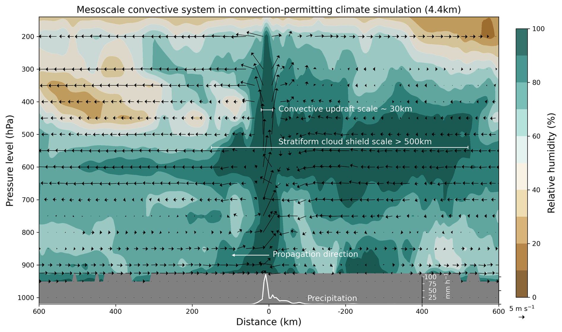
Figure 2 Explicit representation of convective storm circulations in a CP model. We show a simulated convective storm cross-section and for a single timestamp, centred on a storm updraught in a 4.4 km gridbox resolution convection-permitting climate model simulation (CP4-Africa; Senior et al., 2021). The organized storm is visible as an area of > 90 % relative humidity (shading), with extensive cloud anvil across 600–350 hPa pressure levels vertically and extending to a horizontal scale (“x” axis) of > 500 km. Wind vectors indicate a high vertical velocity at the cross-section centre point (0 km), extending across a horizontal scale of approximately 30 km, these being typical features resolvable in this high-resolution CP model but missing in climate models. The resolved updraught circulation is co-located with very high rainfall intensity locally at 0 km (white line, second bottom “y” axis), which rapidly decreases as a function of distance and is specifically linked to the correct representation of the internal updraught circulation. These features of storm processes are expected to be sensitive to the background global warming level (e.g. Prein et al., 2017). A key possibility for AI is to derive equation sets, potentially with stochastic components, that broadly aggregate these complex processes to scales of order 100 km, and so appropriate for inclusion in ESMs

Deriving equation sets via AI brings challenges, first in the large number of input variables that influence convection. While temperature, humidity, wind, and pressure fields may serve as the baseline, derived quantities like convective available potential energy (CAPE) and other vertical profile descriptors, along with spatially variable land characteristics (e.g. topography, vegetation, land use, soil moisture) and oceanic features (e.g. sea surface temperature, surface roughness), significantly impact convective processes. Omitting these variables from new equations could hinder the transferability of knowledge from CP simulations. Moreover, equations must also accurately bridge the scale gap between CP and coarser models, necessitating an algorithm that discovers fundamental relationships transferable to ESM resolutions (e.g. Grundner et al., 2024).

Secondly, while equation discovery offers promise in generating transferable equations for process descriptions beyond their training domain (Ross et al., 2023), it is important to verify they maintain physical consistency and adhere to fundamental principles like moisture and energy conservation. Thus, a question is whether both transferability and physical consistency challenges can be overcome by equation discovery targeting interpretability in ways that other methods cannot achieve. Expert judgement can constrain equation parameters within realistic physical limits, enhancing trustworthiness for extrapolation beyond training conditions (Jebeile et al., 2023). Reliable equations for ESMs that capture convective behaviours will enhance projections of future rainfall extremes in future GHG-enriched environments. Moreover, better constraints on upscale changes in circulation and radiative feedbacks could improve cloud cover modelling in ESMs. A major concern is that some ESMs project very high simulated ECS values, often depending on how they represent climate change feedbacks on cloud features (Bjordal et al., 2020). Dufresne and Bony (2008) provide a detailed disaggregation of direct and feedback drivers (including changes to cloud characteristics) that contribute to simulated global warming as GHGs rise.

As computing power advances, century-long global climate model ensembles at kilometre-scale may become feasible (Slingo et al., 2022), offering more robust projections of convection and related storms as GHG levels rise. However, given the urgent need to understand climate impacts at fine scales, an AI-supported approach is likely invaluable. Equation discovery that captures local effects within a structure available for global calculations may offer an interim solution, reducing resource costs for large ensembles and uncertainty estimation, while providing crucial insights into future rainfall patterns.

3.2 Improving models of terrestrial carbon cycling

We consider modelling large-scale land–atmosphere carbon dioxide (CO₂) exchanges. A substantial fraction of CO₂ emissions are currently absorbed by the ocean and land surface. Whether this continues affects global climate policy, as decreased future natural “drawdown” implies that fewer emissions are compatible with any societal goal to restrict global warming, for example, to 2 °C above preindustrial levels. However, the magnitude of these fluxes, even for the contemporary period, is highly uncertain, despite efforts to constrain it (e.g. Chandra et al., 2022). Budget calculations comparing emissions and atmospheric concentration changes can reveal with high accuracy the combined global land plus ocean CO₂ drawdown and hence offset of emissions. However, Chandra et al. (2022) note (citing Friedlingstein et al., 2020) that the balance between the land and ocean components is unknown within a gigaton of carbon per year. Approaches to reducing uncertainty in regional-to-global land–atmosphere CO₂ fluxes include using FLUXNET towers (e.g. Baldocchi et al., 2001) above strategic representative biomes, atmospheric CO₂ measurements merged with atmospheric transport models generating atmospheric inversions (e.g. Table 1 of Kondo et al., 2020) and forward modelling with dynamic global vegetation models (DGVMs) (e.g. Sitch et al., 2008). Robust forward modelling allows quantifying flux changes expected for any future altered climatic state.

The challenge of simulating the land surface is different from that of the atmosphere. One generalization is that the equations and parameters describing atmospheric processes are well understood but admit rich behaviours, including local convection (Sect. 3.1), which may not be fully understood at large scales. The land surface, however, is modelled with simpler equations, including some components that are algebraic (i.e. not differential equations), but instead, the complexity is substantial heterogeneity in their parameterization. Variation in parameters can be due to multiple factors, including that a typical transect of land will contain many biomes or plant functional types, all having slightly different responses to imposed environmental variations. We propose AI-led approaches that quantify similar processes but recognize different levels of response at finer scales. AI methods may also successfully aggregate such spatial behaviours to generate equation parameters valid at very large scales for inclusion in ESMs.

The eddy covariance method measures high-frequency (many times per second) simultaneous fluctuations in vertical wind speed and a scalar quantity of interest, where their covariance statistic is linearly related to the land–atmosphere exchange of the scalar. There are a growing number of towers with such measurement devices installed on top of them, estimating momentum, heat, vapour, and CO₂ exchanges. The operation of eddy covariance systems and related measurement databases are undertaken by the expanding FLUXNET network (Baldocchi et al., 2001). These measurements already provide training data for ML methods to map from global Earth observation (EO) data products (that record land attributes) to estimates of surface fluxes (Tramontana et al., 2016). This approach, named FLUXCOM, also entrains meteorological measurements at towers as additional driving variables. FLUXCOM then extrapolates tower knowledge using EO and meteorological data, generating global historical estimates of surface energy fluxes (Jung et al., 2019) and CO₂ exchange (Jung et al., 2020).

We consider a slightly different approach to FLUXCOM. Using AI-led equation discovery without prior information will likely generate equations similar to existing knowledge, e.g. for surface energy partitioning (Monteith, 1981) and photosynthesis (Farquhar et al., 1980). However, two (or more) biomes are often in close proximity, which requires the development of “two-source” models (e.g. Huntingford et al., 1995), or descriptions of biomes with complex canopy structures are needed (e.g. Mercado et al., 2007). We suggest an AI-led approach to building models of land–atmosphere CO₂ exchange that is valid at the ESM gridbox scale and accounts for local-scale complexities. We would first use equation discovery methods to model land behaviours at FLUXNET sites. Revised equations would map driving data from EO retrievals that fall within the flux tower footprint (Schmid, 1994), along with FLUXNET meteorological measurements, to the tower data of land–atmosphere CO₂ exchange. Such use of EO supports the suggestions of Chen et al. (2011). AI would derive any equation terms and parameters in addition to standard formulations to capture surface heterogeneity factors. The explicit dependencies on meteorological conditions support creating equations valid for any altered future background climatic conditions.

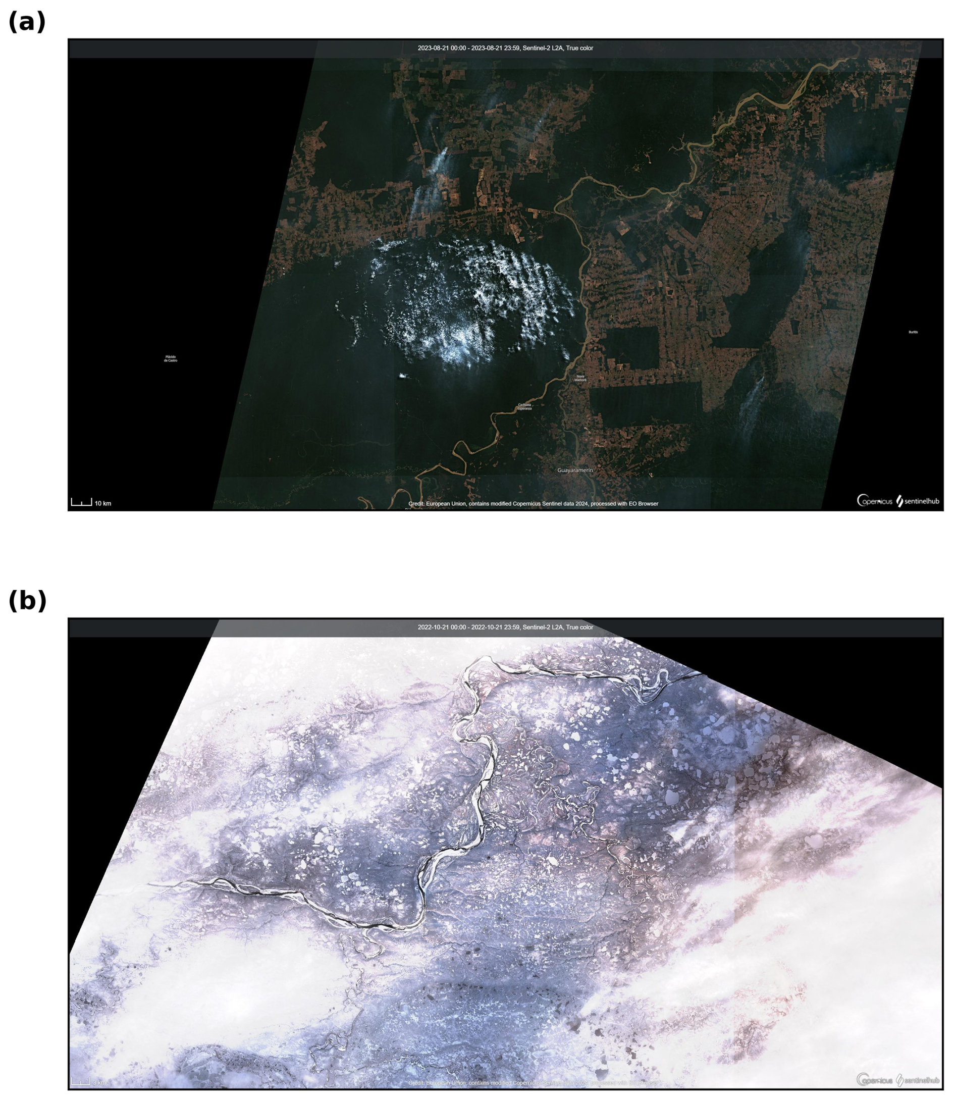
Figure 3 Sentinel-2 L2A images capturing complex land surface information down to 10 m spatial resolution, in this example for (a) deforestation in Rôndonia, Brazil (10° S, 65.7° W), with visible wild fire plumes (please zoom in to see fine-scale land use detail) and (b) a permafrost landscape in Putorana State Nature Reserve, Russia (71° N, 96.3° E) (Copernicus Sentinel-2, 2021). A wealth of high-resolution imagery now documents processes acting on fine-scale land surface patterns and temporal changes therein, opening new avenues for AI-led mapping of sub-grid surface complexity onto physical variables typically used in climate models.

Once established at FLUXNET sites that AI-derived revised equations successfully translate EO measurements to CO₂ exchanges, EO and meteorological data fields can then force these equations elsewhere. Such spatial aggregation of local tower-based calculations to large scales would provide equations with parameters that capture, implicitly, fine spatial heterogeneity in the land surface, offering better ESM-based predictions of CO₂ exchanges. ML-derived spatial aggregation would be a form of technique known as computer vision. In Fig. 3 we present two representative images, panel (a) showing complexity in a tropical rainforest location in South America with extensive land use and (b) of permafrost at high latitude, where there is substantial variation in land attributes. An additional requirement of computer vision algorithms would be that they ignore locations in EO imagery where there are clouds or other masking factors such as smoke from fires (e.g. Fig. 3a).

Our proposed approach would become increasingly accurate as the eddy covariance network extends, noting that Papale (2020) request FLUXNET expansion to support better estimates of global annual land–atmosphere CO₂ exchanges. With more FLUXNET sites, it will be possible to more routinely test discovered equations at a broader range of locations. Where there are discrepancies, this may imply further missing processes in the equation set or a strong regional dependency of parameters, which our techniques may then quantify. As an example, the introduction of geochemical cycles beyond carbon in land models is still in its early stages, with Davies-Barnard et al. (2022) noting major differences in nitrogen cycling representation between ESMs. Furthermore, available data over ever-increasing time periods would allow more testing of whether AI-discovered equations capture climate-induced trends.

3.3 Dynamical system models of ocean circulation

The study of major oceanic circulations is conducted mainly with high-resolution numerical simulations, e.g. ESMs. However, the large computational time of such simulations maintains interest in faster summary models, such as coupled ODEs. Reduced-form operationally fast spatially aggregated bulk ODEs that evolve in time allow researchers to more readily scan parameters and a broader range of future climate forcings, enabling a better assessment of potential features of circulation stability. These simpler dynamical systems can enable levels of understanding not possible with restricted computer power constraining the number of possible perturbed-parameter full-complexity simulations.

Early model attempts at simplified descriptions of oceanic behaviour exist including the Atlantic Meridional Overturning Circulation (AMOC) (e.g. Stommel, 1961). More recently, simplified models have emerged that include atmospheric drivers and their impact on the important El-Niño–Southern Oscillation (ENSO) (e.g. Timmermann et al., 2003). Here, we present the Timmermann model in Fig. 4, in both schematic form (panel a) and bifurcation diagram (panel b), with details in the caption.

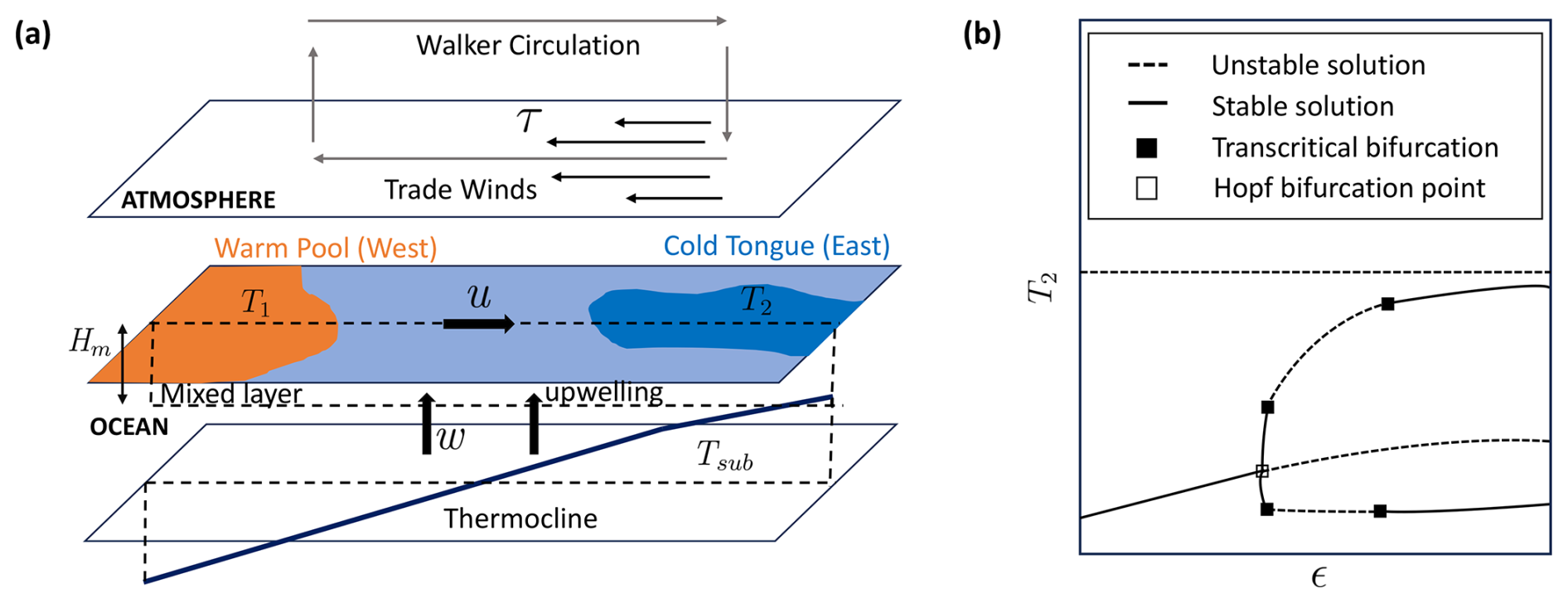
Figure 4 A schematic and bifurcation diagram of the equatorial coupled ocean–atmosphere system as represented in the Timmermann model of ENSO. Panel (a): T₁ (K) and T₂ (K) are the sea surface temperatures of the western Pacific and eastern Pacific respectively, and τ is the wind stress on the ocean surface due to easterly trade winds, given in newtons per metre squared. T_sub (K) is the temperature below the mixed layer of depth H_m (m). The ocean upwelling velocity is denoted w (m s⁻¹), and u (m s⁻¹) is the atmospheric zonal surface wind. Diagram adapted from Dijkstra (2013). Panel (b): bifurcation diagram of eastern Pacific temperature T₂ (K) as a function of zonal advection efficiency ϵ (dimensionless), showing solutions to Eqs. (3) to (4) and their stability. Diagram adapted from Timmermann et al. (2003). We suggest that AI-led equation discovery is well-positioned to investigate oceanic datasets in order to determine if the simplified model presented here remains the most appropriate to maximally represent the ocean–atmosphere system at very large scales.

ENSO is hypothesized to occur as follows. There is a positive ocean–atmosphere feedback process that activates ENSO, first suggested by Bjerknes (1969). The feedback process may start with weakened easterly trade winds, which reduces the strength of the ocean current responsible for drawing surface water away from the western equatorial Pacific. This in turn reduces the ocean upwelling of colder water from the deep ocean, flattening the thermocline. A buildup of warmer surface water in the equatorial east Pacific (El Niño) then emerges. As a result, we now have a reduced east–west sea surface temperature (SST) gradient that further weakens the Walker circulation (a positive feedback mechanism). However, after the El Niño matures, a negative feedback mechanism emerges to turn El Niño into a cold phase known as La Niña. The characteristic timescale of the phase oscillation is 2 to 7 years. In addition, the tropical Pacific SST also exhibits decadal variability related to decadal variations in the amplitude of ENSO (Timmermann et al., 2001; Choi et al., 2012).

When modelling the processes that cause irregular inter-annual El Niño occurrences, there are usually two approaches. The first is deterministic, albeit that there exists chaotic behaviour in the large-scale dynamics of the coupled ocean–atmosphere system due to non-linear interactions. The other viewpoint assumes that this behaviour is only weakly non-linear and the irregular oscillations are mainly due to stochastic noise. The former approach is more suited to using reduced-complexity models of ENSO, which may be gained from using AI-led equation discovery methods to uncover chaotic non-linear dynamics without the need for stochastic terms in the equations.

Modelling the positive and negative feedback mechanisms of ENSO initially led to four basic linear deterministic oscillator models. Such models are known as the delayed oscillator (Suarez and Schopf, 1998), the recharge–discharge oscillator (Jin, 1997), the western Pacific oscillator (Weisberg and Wang, 1997) and the advective–reflective oscillator (Picaut et al., 1997). However, observed ENSO behaviour exhibits non-linear and irregular oscillations which are not accounted for in these simpler models. However, a non-linear ENSO model developed by Timmermann et al. (2003) captures both the inter-annual oscillations and the decadal variability in El Niño events seen in observations and climate models. The details of the physical set-up are given in Jin (1997) and Zebiak and Cane (1987). The heat budget of the Timmermann model is given by two coupled first-order ordinary differential equations in time,

$$\begin{array}{}\text{(3)}& {\displaystyle \frac{\mathrm{d}{T}_{\mathrm{1}}}{\mathrm{d}t}}=-\mathit{\alpha }(T_{\mathrm{1}}-T_{\mathrm{r}})-{\displaystyle \frac{u(T_{\mathrm{2}}-T_{\mathrm{1}})}{L/\mathrm{2}}},\text{(4)}& {\displaystyle \frac{\mathrm{d}{T}_{\mathrm{2}}}{\mathrm{d}t}}=-\mathit{\alpha }(T_{\mathrm{2}}-T_{\mathrm{r}})-{\displaystyle \frac{w(T_{\mathrm{2}}-T_{\mathrm{sub}})}{H_{\mathrm{m}}}},\end{array}$$

where the variables T₁, T₂, T_sub, H_m, w, and u are described in the caption to Fig. 4. The additional variables in Eqs. (3) and (4) are as follows. T_r (K) is the radiation equilibrium temperature in kelvin, L (m) is the basin width, and $\mathrm{1}/\mathit{\alpha }$ (d⁻¹) represents a typical inverse timescale of thermal damping. Furthermore, we have the physically derived relations $\frac{u}{L/\mathrm{2}}=\mathit{ϵ}\mathit{\beta }\mathit{\tau }$ and $w/H_{\mathrm{m}}=-\mathit{\zeta }\mathit{\beta }\mathit{\tau }$, where ϵ and ζ are the strengths of zonal and vertical advection respectively (model bifurcation parameters) and are both dimensionless quantities. The variable β (km⁻¹ s⁻¹) quantifies the strength of the influence of thermocline depth perturbations on SSTs.

The subsurface temperature, T_sub is defined as

$$\begin{array}{}\text{(5)}& T_{\mathrm{sub}}=T_{\mathrm{r}}-{\displaystyle \frac{T_{\mathrm{r}}-T_{\mathrm{r}\mathrm{0}}}{\mathrm{2}}}\left[\mathrm{1}-{\displaystyle \frac{\tanh (H+h_{\mathrm{2}}-z_{\mathrm{0}})}{h_{*}}}\right],\end{array}$$

where T_r0 is the temperature beneath the thermocline; h₂ is the east equatorial Pacific thermocline depth (relative to a depth H) in metres; z₀ is the depth in metres, for which the upwelling velocity w, in metres per second, becomes its characteristic value; and h_* is the sharpness of the thermocline. The thermocline depths are calculated as follows:

$$\begin{array}{}\text{(6)}& {\displaystyle }{h}_{\mathrm{2}}=h_{\mathrm{1}}+bL\mathit{\tau },\text{(7)}& {\displaystyle \frac{\mathrm{d}{h}_{\mathrm{1}}}{\mathrm{d}t}}=-r\left(h_{\mathrm{1}}+{\displaystyle \frac{bL\mathit{\tau }}{\mathrm{2}}}\right),\end{array}$$

where h₁ is the west equatorial Pacific thermocline depth in metres, $\mathrm{1}/r$ (d⁻¹) represents a dynamical adjustment timescale, and b is the efficiency of wind stress τ to drive the thermocline tilt. Wind stress is given by

$$\begin{array}{}\text{(8)}& \mathit{\tau }={\displaystyle \frac{\mathit{\mu }(T_{\mathrm{2}}-T_{\mathrm{1}})}{\mathit{\beta }}},\end{array}$$

where μ (K⁻¹ d⁻¹) is a dynamical coupling coefficient. Overall this leaves us with six equations (Eqs. 3 to 8) and six unknown variables (T₁, T₂, T_sub, h₁, h₂, and τ). For the original parameter values used in this study, see Timmermann et al. (2003). In Timmermann et al. (2003), the bifurcation parameter, ϵ, is varied to understand how the non-linear zonal advection term generates chaotic behaviour.

This low-order model simulates strong decadal El Niño conditions (El Niño bursting) which have been observed in full-complexity simulations, where the ENSO mode grows in amplitude and then quickly resets, from which the amplitude variations grow again. For small values of the zonal advection efficiency bifurcation parameter, ϵ, and a fixed value of ζ, the system is in stable equilibrium with a cold “tongue” in the eastern Pacific and a warm pool in the western Pacific, as shown in Fig. 4a. However, this steady mean state becomes unstable for a larger critical value of ϵ, leading to a Hopf bifurcation, and a stable periodic orbit appears, as illustrated in Fig. 4b. Further analysis (e.g. Fig. 6 in Timmermann et al., 2003) of the dynamical system shows rich behaviour when both ϵ and ζ are varied simultaneously, resulting in ENSO amplitude modulations, period-doubling bifurcations, and chaos.

Relating to the premise of this paper, although the existing simpler models such as that repeated above appear to reproduce many features of ENSO, utilizing AI-led equation discovery offers a potential way to verify this dynamical behaviour using observational datasets and model simulations as training data. Do these newer algorithms back out a model with implicit Hopf bifurcations and low-dimensional chaos that match that found in Timmermann et al. (2003), or will they suggest refinements? We propose the three main potential outcomes of using equation discovery in this context. Firstly, equation discovery may back out simpler deterministic models of ENSO, such as the four basic linear oscillator models mentioned previously. Most of these models can be generalized into a recharge oscillator framework (Jin and An, 1999). Secondly, with careful consideration of the variables and the physical set-up involved, included in Fig. 4, the derived equations may provide verification of the Timmermann model by exhibiting similar non-linear chaotic behaviour for different values of the bifurcation parameters. If this is the case we expect the discovered equations to emulate (1) low-amplitude biannual ENSO oscillations at low values of ϵ, (2) amplitude-modulated and chaotic behaviour at intermediate values of ϵ, and (3) large-amplitude ENSO oscillations with periods of 3–4 years at higher values of ϵ. A third possibility is that the learned equations provide a new description of ENSO behaviour which may potentially come with (1) a better parameterization of the ENSO system, (2) an enhanced understanding of physical mechanisms leading to the generation of non-linear ENSO behaviours which agree better with observations and models, and (3) improved predictive skill of ENSO.

Due to the shortness of available observational records and the level of noise in the data, it can be difficult to determine from observations alone if ENSO amplitude modulations are a statistical manifestation or a result of deterministic processes (Timmermann et al., 2003). AI-led equation discovery methods such as sparse regression only require a limited time series to discover the underlying dynamics and work well in the presence of noise, and they therefore may be effective in this situation.

State-of-the-art ESMs still contain biases in the eastern equatorial Pacific (Timmermann et al., 2018), which leads to problems in representing key physical processes and feedback mechanisms and so may impact their ability to accurately predict future changes. ESMs struggle to converge in their simulations of ENSO characteristics such as amplitude, period, and the asymmetry between El Niño and El Niña phases (Jin et al., 2020). Yet, inter-ESM disagreements are an opportunity for the AI-led discovery of reduced-complexity equations, as such models are computationally fast and thus allow substantial sampling of different parameter values. If such parameters have process interpretations and if it is possible to map ESM projections onto different values of such parameters, this enables the differences and uncertainties between ESMs to be better understood.

4 Discussion and conclusions

AI plays an increasing role in society (e.g. Makridakis, 2017) and will likely influence multiple aspects of scientific research (e.g. Xu et al., 2021). AI methods are proposed to support the mitigation of climate change (e.g. Kaack et al., 2022; Chen et al., 2023; Rolnick et al., 2023) and climate research itself (e.g. Reichstein et al., 2019; Huntingford et al., 2019; Eyring et al., 2024). The basis for most AI algorithms is statistical, frequently introducing non-linearity into forms of regression. For instance Murphy (2013) contains an early chapter on linear regression, to be viewed in the context of subsequent chapters on key AI algorithms. Recently, there has been an emphasis on constraining AI-based discoveries to be compatible with known theory about underlying processes, referred to as “physics-informed AI” (e.g. Karniadakis et al., 2021). An early form of physics-informed activity has been the development and maintenance of data assimilation methods to generate historical gridded datasets of meteorological conditions, e.g. the European Centre for Medium-Range Weather Forecasts ERA5 reanalysis (Hersbach et al., 2020). Reanalysis products merge data with forecasts, balancing the need to simultaneously remain within the uncertainty bounds of measurements and broadly satisfy the equations of atmospheric dynamics.

We propose advancing climate change science with the even newer AI technique of “equation discovery”. Although existing AI methods provide powerful insights into the features of large datasets, they remain essentially statistical and therefore may not estimate well “out of sample”. Yet the main requirement of climate science is to predict environmental regimes different from those of the present day or the recent past. If, instead, AI reveals process equations, this opens the opportunity for their assessment and parameterization. Such an understanding of processes may confirm that the equations have the predictive capability needed to describe new climatic regimes. This supports a fundamental role of applied mathematics in determining data-led equations for a system that can robustly simulate responses to alternative forcings.

Already suggested is using AI to emulate the few limited-area very high-resolution atmosphere simulations and for the forcings for which they have been operated (e.g. Schneider et al., 2023). Such emulators may be placed in ESMs to predict high-resolution atmospheric features, including average storm characteristics, at other locations. Extending such analyses to generate governing equations, possibly with stochastic components, will more rigorously capture high-resolution effects at alternative places and atmospheric GHG levels. Discovered equation sets, amenable to discretization in ESMs, may also simulate small-to-large-scale feedbacks. AI may also enable extending basic equations, allowing additional perturbation term discovery, or location-specific parameters, e.g. for capturing ecological responses with strong spatial heterogeneity. A further application is AI-based discovery of equations that are instead valid over substantial areas (e.g. averaging ESM projections), aggregating geographical variation and reducing to ODEs in time only and that respond to changing GHGs. ODEs are often amenable to more complete analysis, and even if exact solutions are unavailable, they can be tested for linear stability about equilibrium states and for non-linear systems including how parameter perturbation may activate TPs. TPs in the Earth system are the basis for intense research (e.g. Mckay et al., 2022), given their strong potential impacts on society, yet estimated GHG levels causing occurrence are highly ESM-specific (Drijfhout et al., 2015). Mapping to a common simpler model enables characterizing ESMs by effective parameters in such reduced-complexity representations. This approach may identify parts of the Earth system that, if measured better, will better determine GHG levels likely to trigger TPs. Together, factors have led to our three illustrative examples in Sect. 3 of how AI-led “equation discovery” may support climate change science.

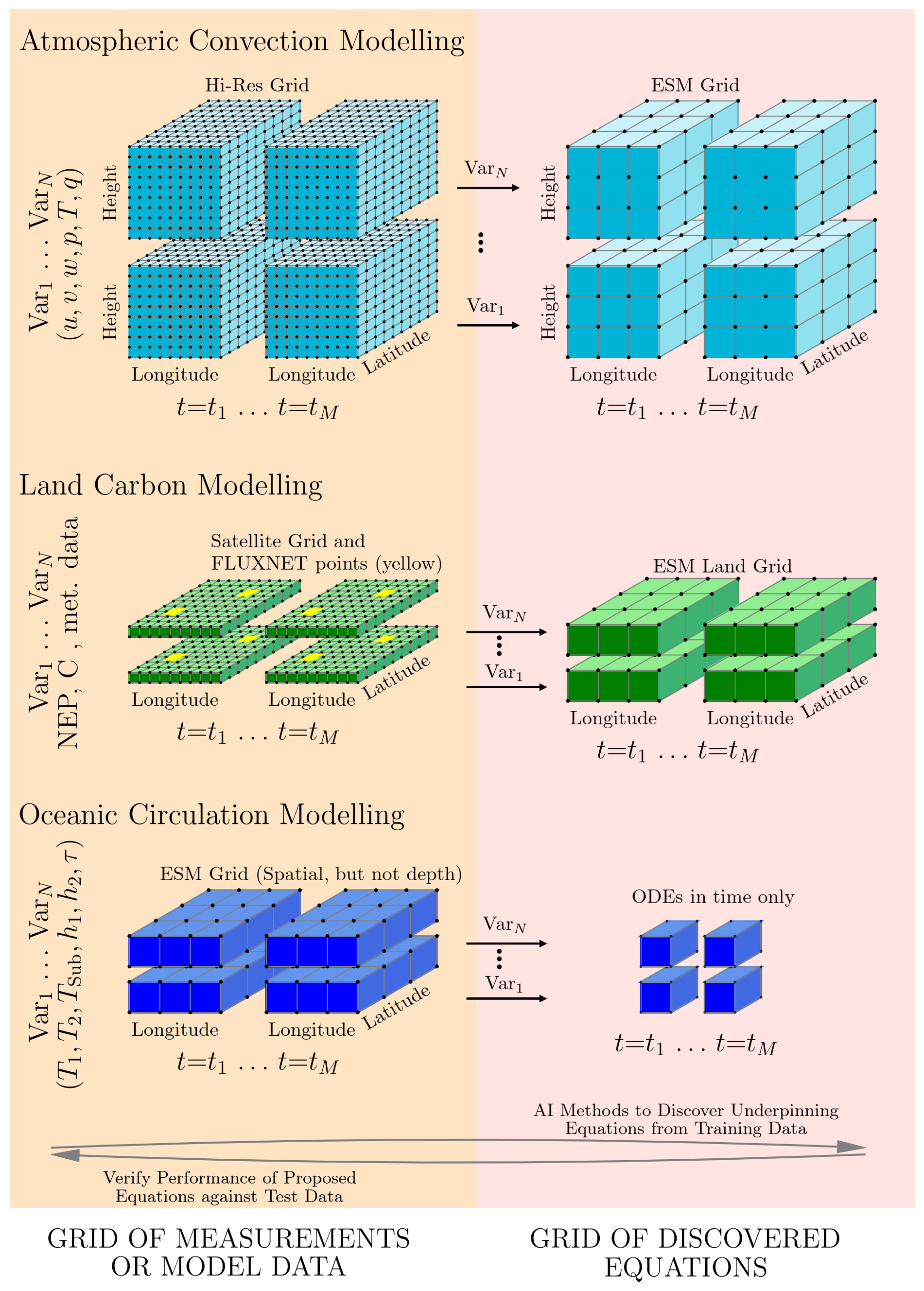
Figure 5 Schematic of the grid of discovered equations. For our three illustrative examples, represented by different rows, the left-hand side shows the numerical mesh of the original data within which AI methods may discover underlying equations. The right-hand side is the potential mesh of such equations. For atmospheric convection, the original data comprise very high-resolution simulated meteorological variables. Each variable is illustrated as different 3-D blocks (vertically) and at different times (horizontally). Derived equations characterizing high-resolution convection would be embedded in existing ESMs on coarser scales, as shown on the top right. Land carbon modelling has two stages. Initially, at specific locations of FLUXNET data (yellow marks), time series of variables related to land–atmosphere carbon exchange, such as net ecosystem productivity (NEP) and meteorological variations, are used to derive time-evolving ODEs. Computer vision methods then calibrate and extrapolate these equations to all locations using high-resolution Earth observation data, ready for placement in the land components of ESMs. Large-scale oceanic circulation modelling would first simply spatially average key depth-independent quantities, T₁, T₂, T_sub, h₁, h₂, and τ, and equations are then found that describe their evolution in time, yielding a reduced-complexity set of ODEs. Not all data would be used in the initial training exercises to determine governing equation sets. As with most AI methods, the remaining data would be used to test algorithms, which here would determine the performance of the proposed equations, hence the right-to-left arrow at the bottom of the diagram. In some instances, there may be repeated cycles around these arrows, with alternative sets of equations derived for consideration and appropriate methods selected to compare them (e.g. the Akaike information criterion, AIC, statistics).

The three examples are (i) simulation of atmospheric convection, which solves equations at very high resolution (∼ 1 km grid) to represent the spatial heterogeneity of individual storms. Such models have high computational demands, which limits them in the range of modelled spatial extent and GHG concentrations. The goal is to develop from these calculations “bulk” differential equations suitable for ESMs operating at coarser (∼ 100 km) grids. These new equations need to aggregate fine-scale dynamics and their interactions with boundary conditions, simulate feedbacks where appropriate on ESM-simulated large-scale dynamics, and may incorporate stochastic components to describe the intensity and duration of convective events at fine scales. (ii) The second is the simulation of terrestrial carbon cycling. The fundamental equations governing land–atmosphere CO₂ exchange due to photosynthesis and respiration are known and routinely included in ESMs. However, at local scales, the parameterization of these equations strongly depends on biome type. Additional terms may need derivation for complex canopy structures or where different biomes are close and have key within-canopy interactions. These factors may aggregate to impact ESM-scale parameterizations; hence the challenge is two-fold. The first is to calibrate and, where necessary, discover new equation terms for key or co-located biomes, possibly guided by eddy-covariance measurements. The second is to utilize AI methods to entrain Earth observation data, enabling spatial aggregation beyond flux towers to generate equations and parameters applicable at ESM gridbox scales. This suggestion will improve ESMs with interactive carbon cycle simulations, providing better assessments of the extent to which the land surface will partially offset future CO₂ emissions. (iii) The last is the large-scale summary simulation of ocean currents. This proposed AI application would derive globally applicable reduced-complexity ocean models from ESMs, offering several uses. A simpler model can explore responses to wide ranges of future emissions trajectories not possible with full ESMs due to their computational constraints. Reduced-complexity models facilitate parameter scanning and, in the case of non-linearity, build on dynamical systems theory to illustrate any potential for TP occurrence. Fitting simpler model parameters to each member within an ESM ensemble allows improved characterization of inter-ESM variations and thus uncertainties. Finally, newer AI-derived reduced-complexity equations, drawn from data or ESMs, may reveal if current simpler models, such as the Timmermann ENSO model, continue to be appropriate or if alternative versions of oscillator models are more valid. To capture at least some of the aspects of the potential sets of AI-derived equations, in Fig. 5 we present the numerical mesh of original models and data (left-hand side) and the grid for new equations (right-hand side).

It is easier to set aspirations for implementing AI methods in climate science than to actually perform the analysis itself. Some of the suggestions here are likely major research projects that could take multiple years to complete. However, with the rapid pace of algorithm development raising questions about applicability to climate research, we aim to highlight the particular method of equation discovery. We contend that equation discovery, a form of interpretable AI, may substantially enhance some aspects of climate research that traditional analytical, statistical, or other AI methods may not address. An emphasis on equation development, and their inherent description of processes, allows moving on from the complaint that AI-developed models are purely statistical and may fail if extrapolated to make predictions for higher future GHG levels (although some capability of statistical AI methods to predict new forcings is noted by Scher and Messori, 2019). Although an initial set of equations might also be suspected to have poor “out-of-sample” performance, their existence provides a stronger basis for interpreting processes and interactions. Subsequent careful fitting of equation parameters may generate robust predictive capability.

ESMs will almost certainly remain the primary tool for advising climate policy, and two of our examples (modelling convective storms and terrestrial carbon cycling) offer the possibility of improving the reliability of such models. Better aggregation of subgrid storm process representation to ESM gridbox scale may remove known issues with existing cloud representations (Randall et al., 2003). The current variation in proposed subgrid atmosphere and land parameterizations may contribute to the large inter-ESM differences in the projection of changes in rainfall patterns (e.g. Yazdandoost et al., 2021) and the global carbon cycle (e.g. Huntingford et al., 2009) respectively. Improving emulation of subgrid effects in ESM development aligns with the commentary of Wong (2024) on AI and climate, although we again stress the retention of process understanding allowed through equation representation.

Could AI replace conventional climate research? This question is already being asked about weather forecasting (e.g. Schultz et al., 2021). AI has shown skill in predicting severe weather events (e.g. Bi et al., 2023; Lam et al., 2023), but McGovern et al. (2017) argue that it remains essential to continue developing, in parallel, a physical understanding of high-impact meteorological events. A deeper understanding of the balance of dominant equation terms, possibly determined by AI, may reveal causal links between processes during the preceding periods of extreme events (“storylines”; Shepherd, 2019) and therefore support earlier warnings. We suggest that AI employed for equation discovery will actually engage climate research scientists further rather than creating any form of replacement. Although climate change is mainly simulated with ESMs, their ability to offer ever more refined estimates of change is arguably at a plateau. For similar future pathways in GHGs, the spread of projections between the models in version 5 of the Climate Model Intercomparison Project (CMIP5) and the more recent version 6 (CMIP6) has not decreased for the basic quantities of changes in global mean temperature and global mean precipitation (e.g. Fig 4 of Tebaldi et al., 2021). Reflecting on our three illustrative but specific examples (Sect. 3.1, 3.2, and 3.3), we conjecture that the particular form of AI that is the discovery of equations may lower uncertainties in ESMs and for both their regional and global projections. These reductions will be by (i) providing new robust equations that capture subgrid processes, (ii) creating valid grid-scale parameterizations for existing equations that aggregate fine-scale processes, and (iii) disentangling complex processes to equation sets far simpler than ESMs but that capture the dominant processes. The latter simpler equations may guide measurement programmes towards tuning key parameters, and where such knowledge ultimately feeds back by improving ESM parameter calibration.