Impacts of North American forest cover changes on the North Atlantic Ocean circulation

Planetary-scale forestation has been shown to induce global surface warming associated with a slowdown of the Atlantic Meridional Overturning Circulation (AMOC). This AMOC slowdown is accompanied by a negative North Atlantic sea surface temperature (SST) anomaly resembling the known North Atlantic warming hole found in greenhouse gas forcing simulations. Likewise, a reversed equivalent of the SST response has been found across deforestation experiments. Here, we test the hypothesis that localised forest cover changes over North America are an important driver of this response in the downstream North Atlantic Ocean. Moreover, we shine a light on the physical processes linking forest cover perturbations to ocean circulation changes. To this end, we perform simulations using the fully coupled Earth system model CESM2, where pre-industrial vegetation-sustaining areas over North America are either completely forested (“forestNA”) or turned into grasslands (“grassNA”). Our results show that North American forest cover changes have the potential to alter the AMOC and North Atlantic SSTs in a manner similar to global ones. North American forest cover changes mainly impact the ocean circulation through modulating land surface albedo and, subsequently, air temperatures. We find that comparably short-lived cold-air outbreaks (CAOs) play a crucial role in transferring the signal from the land to the ocean. Around 80 % of the ocean heat loss in the Labrador Sea occurs within CAOs during which the atmosphere is colder than the underlying ocean. A warmer atmosphere in forestNA compared to the “control” scenario results in fewer CAOs over the ocean and thereby reduced ocean heat loss and deep convection, with the opposite being true for grassNA. The induced SST responses further decrease CAO frequency in forestNA and increase it in grassNA. Lagrangian backward trajectories starting from CAOs over the Labrador Sea confirm that their source regions include (de-)forested areas. Furthermore, the subpolar gyre circulation is found to be more sensitive to ocean density changes driven by heat fluxes than to changes in wind forcing modulated by upstream land surface roughness. In forestNA, sea ice growth and the corresponding further reduction in ocean-to-atmosphere heat fluxes forms an additional positive feedback loop. Conversely, a buoyancy flux decomposition shows that freshwater forcing only plays a minor role in the ocean density response in both scenarios. Overall, this study shows that the North Atlantic Ocean circulation is particularly sensitive to upstream forest cover changes and that there is a self-enhancing feedback between CAO frequencies, deep convection, and SSTs in the North Atlantic. This motivates studying the relative importance of these high-frequency atmospheric events for ocean circulation changes in the context of anthropogenic climate change.

1 Introduction

Forests provide habitats for numerous species, offer valuable ecosystem services, and act as carbon sinks. The latter makes afforestation and reforestation (hereafter summarised with the term forestation) an attractive carbon mitigation strategy, alongside minimising carbon emissions, to combat global temperature rise (Mo et al., 2023; Rohatyn et al., 2022; Bastin et al., 2019). In addition to absorbing carbon from the atmosphere, forestation locally promotes evapotranspiration and shading from direct shortwave radiation, decreases surface albedo, and increases surface roughness, while deforestation has the opposite effect (Bonan, 2008; Mahmood et al., 2014). The influence of these so-called biogeophysical effects extends beyond the local scale and can have significant impacts in remote areas (Portmann et al., 2022; Hua et al., 2023; Snyder, 2010; Swann et al., 2012). In particular, albedo changes following forestation contribute to warming at the global scale, while the albedo effect of deforestation contributes to cooling (De Hertog et al., 2023; Portmann et al., 2022; Winckler et al., 2019; Jiao et al., 2017; Davin and de Noblet-Ducoudre, 2010; Snyder et al., 2004). Depending on the considered region, the albedo effect of large-scale forestation or deforestation can partly or fully offset the carbon effect (Weber et al., 2024; Jayakrishnan and Bala, 2023; Bonan, 2008; Bala et al., 2007; Renssen et al., 2003; Betts, 2000). The dominating effect depends heavily on latitude. While large-scale forestation in the tropics tends to have a net cooling effect (carbon and evapotranspiration effects dominating), boreal forestation leads to a net warming on the global scale (albedo effect dominating), and vice versa for deforestation (Rohatyn et al., 2022; Windisch et al., 2021; Li et al., 2015; Wang et al., 2014; Betts, 2000). Moreover, the response to extreme high-latitude forest cover changes was shown to differ between continents in the past, with North America showing a comparably strong albedo response (Guo et al., 2024; Asselin et al., 2022).

Beyond the named biogeophysical effects, forestation has been found to also induce anomalies in sea surface temperatures (SSTs). Yet, of the above studies, only some incorporated a dynamic ocean model response to forest cover changes (Guo et al., 2024; De Hertog et al., 2023; Hua et al., 2023; Portmann et al., 2022; Davin and de Noblet-Ducoudre, 2010; Wang et al., 2014; Winckler et al., 2019; Bala et al., 2007; Snyder et al., 2004; Renssen et al., 2003), and of those, a limited number have thus far analysed the ocean response (Guo et al., 2024; Jayakrishnan and Bala, 2023; Portmann et al., 2022; Davin and de Noblet-Ducoudre, 2010; Bala et al., 2007; Renssen et al., 2003). However, in several of these land use change experiments that adopted a dynamic ocean, the North Atlantic Ocean featured a SST anomaly of the opposite sign to the surrounding land and ocean, i.e. a local cooling in an otherwise warmer surrounding environment, and vice versa (Guo et al., 2024; De Hertog et al., 2023; Boysen et al., 2020; Davin and de Noblet-Ducoudre, 2010; Bala et al., 2007). The emergence of such SST anomalies is herein referred to as a North Atlantic warming hole (NAWH) for a cool anomaly, as adopted in the literature addressing North Atlantic Ocean variability (Keil et al., 2020; Gervais et al., 2018), and as a North Atlantic cooling hole (NACH) for the opposite phenomenon. However, the underlying drivers of the NAWH and NACH have not been further explored in these studies.

The NAWH is also a prominent feature in future climate projections and in observations over the last century (Rahmstorf et al., 2015; Keil et al., 2020; He et al., 2022; Liu et al., 2020; Menary and Wood, 2018). Its emergence has been linked to changes in ocean circulation, in particular the Atlantic Meridional Overturning Circulation (AMOC) (Gervais et al., 2018; Caesar et al., 2018; Rahmstorf et al., 2015; van Westen et al., 2024; Ditlevsen and Ditlevsen, 2023; Rahmstorf, 2002; Armstrong McKay et al., 2022; Keil et al., 2020). Conceptually, in the subpolar North Atlantic, a warmer boreal atmosphere leads to reduced heat loss of the ocean to the atmosphere, which results in decreased deep-water formation (DWF) and AMOC strength (Liu et al., 2020; Keil et al., 2020). This leads to reduced transport of heat and salt into the North Atlantic, as well as a reduced mixing of warmer waters from below (Gelderloos et al., 2012; Drijfhout et al., 2012; Menary and Wood, 2018; Putrasahan et al., 2019; Keil et al., 2020). Consequently, upper-ocean heat content reduces (Stolpe et al., 2018), which is linked to reduced SSTs (Rahmstorf et al., 2015). The reduced SSTs can, in turn, be a positive feedback on AMOC slowdown through enhanced sea ice growth and subsequent insulation from the atmosphere that leads to cooler SSTs. Cooler SSTs result in the formation of a NAWH in a warmer climate. However, the relationship between AMOC strength and NAWH has been found to be strongly non-linear (Keil et al., 2020).

Moreover, as the second large-scale ocean circulation pattern in the North Atlantic, the subpolar gyre circulation also modulates the transport of salty waters and thus DWF and the NAWH (Keil et al., 2020; Fan et al., 2021; Böning et al., 2023; Gervais et al., 2018; Liu et al., 2019). Recently, underlying atmospheric drivers of DWF and the SST anomalies have received more attention. Changes in wind stress have been found to play an important role by modulating the subpolar gyre and subsequently DWF, resulting in positive and negative SST anomalies (Putrasahan et al., 2019; Hu and Fedorov, 2020; Lohmann et al., 2021). Moreover, DWF has been connected to so-called cold-air outbreaks (CAOs), which are transient weather events during which the ocean is significantly warmer than the atmosphere (Papritz et al., 2015; Papritz and Spengler, 2017; Papritz and Grams, 2018; Holdsworth and Myers, 2015). Observational data suggest that heat fluxes during CAOs play a central role in buoyancy reduction in the surface waters in DWF sites (Svingen et al., 2023).

A recent study (Portmann et al., 2022) investigated the climate response to global-scale forest cover changes and focused on the role of the global atmosphere and ocean circulation. Using the Community Earth System Model (CESM) version 2, the authors found a NAWH accompanied by a decrease in the AMOC strength in response to global warming induced by large-scale forestation. Conversely, global deforestation resulted in a NACH and long-term increases in the AMOC strength with respect to a control simulation. Another recent study (Guo et al., 2024) performed deforestation experiments for each continent. Their North American and Eurasian vegetation removal experiments, conducted with CESM version 1, also showed a prominent cooling hole in the North Atlantic. However, the physical mechanisms responsible for these changes in ocean circulation in response to forest cover changes remain open.

The objective of this study is to explore the impact of North American forest cover changes first on the atmosphere, then on atmosphere–ocean interactions downstream of North America, and ultimately on the ocean circulation. Given the strong sensitivity of the North Atlantic Ocean to climate forcing, we test the hypothesis that forest cover changes over the upstream continent, i.e. North America, play a crucial role in the downstream ocean circulation, including SSTs. More specifically, we investigate the following research questions.

• How sensitive is the North Atlantic Ocean to upstream forest cover changes in comparison to global forest cover changes?

• What mechanisms related to buoyancy and wind forcing play a role in modulating the North Atlantic Ocean circulation in North American forestation and deforestation scenarios?

• How does a regional warming or cooling on land propagate downstream over the ocean and shape the response of the ocean circulation?

To answer these questions, we analyse fully coupled Earth system model simulations performed with CESM version 2, featuring pre-industrial CO₂ levels, in which vegetation-sustaining areas are either fully forested or deforested north of 30° N latitude over the North American continent. Moreover, we perform Lagrangian trajectory analysis to trace the signal propagation from North American land into the North Atlantic Ocean. Throughout this work, we aim to contextualise our findings in the broader picture of atmosphere–ocean dynamics in the subpolar North Atlantic. In particular, we compare our results to future climate simulations concerning ocean circulation changes and the NAWH and discuss the potential transferability of our conclusions regarding the identified physical mechanisms.

The paper is structured as follows: first, we introduce the setup of our forestation and deforestation experiments and the methods needed for the analyses in Sect. 2. Subsequently, we present the response of near-surface temperature, wind, and AMOC strength and compare this response to North American forest cover changes to global forestation scenarios previously published by Portmann et al. (2022) in Sect. 3.1. The following sections will explore how the found changes in temperature and wind over land drive the changes in the ocean circulation. They are structured as follows: the mechanisms controlling the buoyancy forcing in Sect. 3.2, the trajectory analysis in Sect. 3.3, and the impact of wind forcing on the ocean in Sect. 3.4. The results are summarised and discussed in Sect. 4 and complemented by ideas for further research.

2 Methods

2.1 Model setup

This study is based on simulations using CESM version 2.1.2 (Danabasoglu et al., 2020a), using the Community Atmosphere Model (CAM6) and the Community Land Model (CLM5), the Parallel Ocean Program (POP2), the Los Alamos National Laboratory Sea Ice model (CICE5), and the hydrological routing Model for Scale Adaptive River Transport (MOSART). We perform three simulations, namely a pre-industrial control run, hereafter referred to as “control”; a forested run, “forestNA”; and a deforested run, “grassNA”. The implementation of the forest cover changes is the same as in Portmann et al. (2022) and was first developed by Davin et al. (2020). Vegetation-sustaining areas, here referring to all areas without deserts (e.g. Sahara), ice deserts (e.g. Greenland), or urban areas, are forested for forestNA, while all pre-industrial vegetation is converted to grassland in grassNA. In contrast to the approach in Portmann et al. (2022), forestation and deforestation are confined to North America and taken as all ice-free grid points between 30 and 85° N and between 170 and 50° W (Fig. B1a, b). The implementation of forest cover changes is of an idealised nature, as it does not take present-day land use into account. Therefore, the large croplands in North America are fully forested in these simulations. It should thus not be considered a realistic forestation scenario (such as Griscom et al., 2017; Bastin et al., 2019; Mo et al., 2023) but as an idealised forestation experiment confined to a specific region in favour of exploring the governing mechanisms of the climate response.

In forestNA, areas with especially high forest cover changes are located from Alaska to northern Quebec, Newfoundland and Labrador, and the Great Plains (Fig. B1a). North American deforestation is most pronounced on the northwestern coast and in a band north of the Great Plains up to southern Quebec and the northeastern USA (Fig. B1b). Atmospheric CO₂ concentrations are held constant at pre-industrial levels to isolate the biogeophysical effects of forest cover changes in opposition to carbon cycle effects. The land model is run in the dynamical biogeochemistry mode. Therefore, forestation does not always translate into mature trees in especially dry (e.g. Great Plains) or cold (e.g. Arctic islands) regions. Therefore, we show the mean canopy-top height 50 to 300 years after the model initialisation as an indicator of realised forest cover changes (Fig. B1c, d). Note also that boreal regions are largely populated by shrubs (compare Fig. 1 in the supplement of Portmann et al. (2022)), which are also removed in grassNA. This leads to a notable increase in albedo without large changes in forest cover or canopy height (Fig. B1f).

The simulations are performed at a horizontal resolution of 1°. The three aforementioned experiments are branched off from a 1000-year pre-industrial control run after 200 years of spin-up time and subsequently run for 300 years. We note that the North Atlantic is anomalously fresh and cold, with large AMOC variability (around −3 to +4 standard-deviations; not shown) at and around the branching point. This could bias the sensitivity of the North Atlantic to forest cover changes but is assumed to be of minor importance as the AMOC response to forest cover changes is shown to be larger than this variability (Fig. 2c). In addition, another forestation simulation branched off 50 years later features a similar, if not faster, AMOC response (not shown). The following results are presented for the years 50 to 300 of the experiments and are referred to as the long-term response, unless otherwise stated. We note that depending on the definition of equilibrium, one could argue that an equilibrium state of the ocean circulation can take several millennia to establish (van Westen and Dijkstra, 2023; Curtis and Fedorov, 2024). We, however, are interested in the mechanisms driving the response of the ocean circulation on a centennial timescale that is similar to studies focusing on anthropogenic climate change (Rahmstorf et al., 2015; Liu et al., 2020; Keil et al., 2020).

It is important to note that recent studies have found considerable model dependency of the climate response to vegetation changes. De Hertog et al. (2023) have shown that CESM reacts to afforestation with a stronger warming over land and stronger cooling in the North Atlantic than two other models (the Max Planck Institute for Meteorology Earth System Model (MPI-ESM) and the European Consortium Earth System Model (EC-EARTH)) they compared. Notably, the two other models showed no cooling in the North Atlantic. De Hertog et al. (2024) showed similar model dependencies for the atmospheric water cycle. On the other hand, Boysen et al. (2020) explored the reaction of several CMIP6 models to idealised global deforestation. In their analysis, six of the nine models analysed show a cooling hole, and the global mean temperature response of CESM is close to the model mean. Moreover, CESM has been shown to simulate more DWF in the Labrador Sea and is more sensitive to changes in the Labrador Sea than has been historically observed (Gervais et al., 2018; He et al., 2022).

2.2 Statistical significance testing

To test the statistical significance of the differences between the two experiments (forestNA and grassNA) and the control run, we employ the same approach as in Portmann et al. (2022). A two-sided Wilcoxon rank sum test (Wilks, 2011) is applied to the time series of annual or seasonal means in the considered period on each grid cell separately. The null hypothesis tested is that a randomly drawn value from the experiment time series is equally likely to be larger or smaller than a randomly drawn value from the control time series. To control for the false discovery rate when testing multiple hypotheses on a field, we employ a Benjamini–Hochberg correction (Wilks, 2016), with the false discovery rate set to α_FDR=0.05.

2.3 Buoyancy flux decomposition

The buoyancy of ocean water, given by −gρ (g is the acceleration due to gravity; ρ is the density) is modulated by salinity and temperature (Gill, 1982). Less dense waters are hence more buoyant, and a positive buoyancy flux anomaly (here defined as positive upwards) means water becomes more buoyant. In this study, buoyancy flux is given in kg m⁻² yr⁻¹. To connect near-surface atmospheric variability to the thermodynamic state of the ocean, we calculate the changes in buoyancy at the surface. Ocean salinity changes result from freshwater fluxes and temperature changes from heat fluxes through the ocean surface. The buoyancy flux into or out of the ocean B thus reads

$$\begin{array}{}\text{(1)}& B=B_{\mathrm{H}}+B_{\mathrm{FW}}={\displaystyle \frac{\mathit{\alpha }}{c_p^{\mathrm{water}}}}Q+\mathit{\beta }{\mathit{\rho }}_{\mathrm{S}}\cdot S\cdot F_{\mathrm{FW}},\end{array}$$

with B_H as the buoyancy flux related to heat and B_FW as the flux related to freshwater. The heat-related flux is given by the thermal expansion coefficient $\mathit{\alpha }=-{\mathit{\rho }}^{-\mathrm{1}}\frac{\partial \mathit{\rho }}{\partial T}$ in K⁻¹, the specific heat content of water is $c_p^{\mathrm{water}}$, and the heat flux is Q. The freshwater-related buoyancy flux is the product of the haline contraction coefficient $\mathit{\beta }={\mathit{\rho }}^{-\mathrm{1}}\frac{\partial \mathit{\rho }}{\partial S}$ in kg g⁻¹, the density of salt water is ρ_S, and the sea surface salinity (SSS) is S in g kg⁻¹, with the fresh water flux as F_FW (Pellichero et al., 2018). For the values of the constants and the remaining units of the variables above, refer to Table A1. We assume $c_p^{\mathrm{water}}$ and ρ_S to be constant to simplify and speed up the computation of the buoyancy fluxes. Regarding the haline and thermal expansion coefficient, Gelderloos et al. (2012) found a feedback of the thermal expansion coefficient on the decline in AMOC during the Great Salinity Anomaly from 1968 to 1971, which is why we compute α and β as functions of local salinity, temperature, and sea level pressure, according to IOC et al. (2010), using the gsw-python library (McDougall and Barker, 2011).

We separate radiative (B^rad), turbulent (B^turb), and extracted heat due to snowmelt and ice melt, including latent-heat-related ($B^{{\mathrm{melt}}_{\mathrm{H}}}$) components that are the heat-related contributions to the buoyancy flux. The freshwater-related flux is split into a flux resulting from ice melt ($B^{{\mathrm{ICE}}_{\mathrm{FW}}}$) and one containing the fluxes from precipitation (containing snow), evaporation, and river runoff (B^PERO). The detailed computation of these fluxes from model output variables can be found in the Appendix (Sect. A1). For the analysis of buoyancy fluxes, we use monthly averaged model outputs.

2.4 Identification of cold-air outbreaks

CAOs are events of a positive temperature difference between the ocean surface and the overlying atmosphere. These events lead to a large heat flux from the ocean to the atmosphere, ocean cooling, and subsequently DWF (Holdsworth and Myers, 2015; Papritz et al., 2015). Similar to Papritz and Grams (2018), we identify CAOs as grid cells, where the difference Δθ (in K) between the potential skin temperature θ_SKT (K) and potential temperature at 850 hPa θ₈₅₀ (K) is larger than 0, with $\mathrm{\Delta }\mathit{\theta }={\mathit{\theta }}_{\mathrm{SKT}}-{\mathit{\theta }}_{\mathrm{850}}$. Using the skin temperature is beneficial, since it is also defined over ice. It is computed as follows:

$$\begin{array}{}\text{(2)}& {\mathit{\theta }}_{\mathrm{SKT}}=T_{\mathrm{S}}{\left({\displaystyle \frac{p_{\mathrm{ref}}}{p_{\mathrm{S}}}}\right)}^{\left(\frac{R}{c_p^{\mathrm{air}}}\right)}.\end{array}$$

Here, T_S is the surface temperature given by the model output in K; p_ref= 1000 hPa; p_S is the surface pressure (in hPa); $R/c_p^{\mathrm{air}}=\mathrm{0.268}$, with R as the gas constant (in J mol⁻¹ K⁻¹); and the specific heat of the air $c_p^{\mathrm{air}}$ (in J kg⁻¹ K). Since CAOs are often short-lived, they are identified using 6-hourly atmospheric model output. Similar to Papritz and Spengler (2017), CAO regions are categorised according to the magnitude of Δθ in (0,4], (4,8], (8,12], and > 12 K. The resulting CAO masks include, for example, the centre of a CAO of 9 K in the (8,12] K category. Surrounding this centre, there is an area in the (4,8]K category, which, in turn, is surrounded by an area in the (0,4] K category.

These binary CAO masks are subsequently used to mask heat fluxes in the Labrador Sea – here defined from 52 to 65° N and from 45 to 65° W (see the black box in Fig. 3m). The resulting masked heat fluxes are summed up in time and space and divided by the total upward heat flux in the Labrador Sea. This gives the fraction of positive upwards heat flux associated with CAOs with respect to the total heat flux in this area. Moreover, the resulting two-dimensional CAO fields are used to identify potential target regions for trajectory analysis in Sect. 3.3. For the trajectory analysis, we refer to CAOs with Δθ≤ 8 K as weak CAOs, while CAOs with Δθ>8 K are referred to as strong CAOs.

2.5 Trajectory analysis

Lagrangian air parcel trajectories are computed to trace the impact of forest cover change on the ocean using 6-hourly model output. The 5 d backward trajectories are started every 12 h, 100 km apart, and 100 hPa above the ground in the Labrador Sea, where $\mathrm{\Delta }\mathit{\theta }={\mathit{\theta }}_{\mathrm{SKT}}-{\mathit{\theta }}_{\mathrm{850}}>$0 K. The extent of the Labrador Sea and thereby target region is defined as in Sect. 2.4. Land areas are excluded from the starting points. We post-process the trajectories, filtering out trajectories with a Δθ below the CAO threshold, since some trajectories might be started outside the masks due to grid interpolation. The trajectories are computed using Lagranto version 2.0 (Sprenger and Wernli, 2015) adapted to use CESM output. For this analysis, 6-hourly model output from the years 150 to 200 is used. We restrict this analysis to 50 years to reduce computational costs since we do not expect a qualitative change in our results by including more years. The window of the years 150 to 200 is a time period of relatively stable AMOC strength in forestNA and grassNA (Fig. 2c). Along the trajectories, several variables are traced, namely the potential temperature of the air parcel, potential skin temperature below the trajectory, and net surface turbulent heat fluxes.

Starting the trajectories in CAO regions in the Labrador Sea allows the tracing of the impact of forest cover change on the ocean circulation through the effect on the connecting air parcels. The evolution of the traced variables from CAO trajectories is compared between forestNA and grassNA for strong and weak CAO target regions. Normalised trajectory densities are first presented in Sect. 3.3, following the approach of Schemm et al. (2016), and are calculated as $\frac{n_i}{N_{\mathrm{t}}{\mathrm{area}}_i}\cdot \mathrm{100}$, with n_i as the number of trajectories associated with a certain grid cell i, N_t as the total number of trajectories existing at time step t, and area_i as the area of the concerned grid cell (in km²). The unit of the density is % km⁻².

2.6 Wind-driven streamfunction

To estimate the effect of wind stress changes on the direction of the oceanic flow, we calculate a simple approximation of the wind-driven flow using the Sverdrup relation (Sverdrup, 1947),

$$\begin{array}{}\text{(3)}& V_{\mathrm{Sv}}={\displaystyle \frac{\mathrm{1}}{{\mathit{\rho }}_{\mathrm{0}}\mathit{\beta }}}\mathrm{\nabla }\times \left(\mathit{\tau }\right),\end{array}$$

where V_Sv is the depth-integrated meridional transport, ρ is the density of seawater, β is the Rossby parameter (in m⁻¹ s⁻¹), and τ is the surface wind stress (in Pa) from model output. Here ∇×(τ) denotes the curl of the wind stress vector field. This is then zonally integrated from the eastern boundary to yield a streamfunction related to wind stress forcing. We note that this can only provide a very rough estimate and should not be overinterpreted since the Sverdrup balance is not fully accurate in the subpolar North Atlantic (Wunsch and Roemmich, 1985; Yeager, 2015). Discrepancies between the estimate of the wind-driven circulation and the actual barotropic flow arise mainly due to the complex bathymetry and can locally be on the order of 100 % (Yeager, 2015). However, we argue that changes in the wind-driven streamfunction would have to be comparable to changes in the barotropic streamfunction (averaged across the subpolar North Atlantic) if wind were the dominant driver of subpolar gyre circulation changes. While more sophisticated methods exist (e.g. Chen et al., 2022), we follow other previous studies using this approach for comparability (Putrasahan et al., 2019; Lohmann et al., 2021; Ghosh et al., 2023).

3 Results

First, the long-term response of surface variables and AMOC to North American forestation and deforestation is described. These are related to the global-scale simulations discussed in Portmann et al. (2022) to investigate the sensitivity of the North Atlantic to upstream forest cover changes. Moreover, similarities and differences in the found long-term response to anthropogenic warming simulations are explored. This is followed by a more in-depth analysis of air–sea interactions, which are grouped into thermodynamic processes (including CAOs) and the trajectory analysis, followed by the mechanical processes (wind stress).

3.1 Response of near-surface temperature, wind, and the Atlantic Meridional Overturning Circulation

We find that North American forestation warms global mean near-surface temperatures by 0.09 K, while deforestation cools it by 0.52 K (Fig. 1a, b). As expected, the temperature changes are most pronounced over North American land. However, the North Atlantic near-surface temperatures cool by more than 4 K regionally in forestNA and warm by up to 1 K in grassNA. In forestNA, the negative anomaly near the North Atlantic Ocean surface extends downstream over Europe with still significant cooling in North Africa, as well as regions east of the Caspian Sea and eastern China. Large parts of the Southern Hemisphere exhibit a slight warming response. This points towards a decrease in meridional overturning and thus less equatorward heat export from the Southern Ocean (Rahmstorf, 2024; Armstrong McKay et al., 2022). In contrast, deforestation significantly cools the Northern Hemisphere and large parts of the Southern Hemisphere. Cooling is most pronounced over the deforested areas. Similar to forestNA, the response of the Southern Hemisphere in grassNA is likely related to an increase in equatorward ocean heat transport further described below.

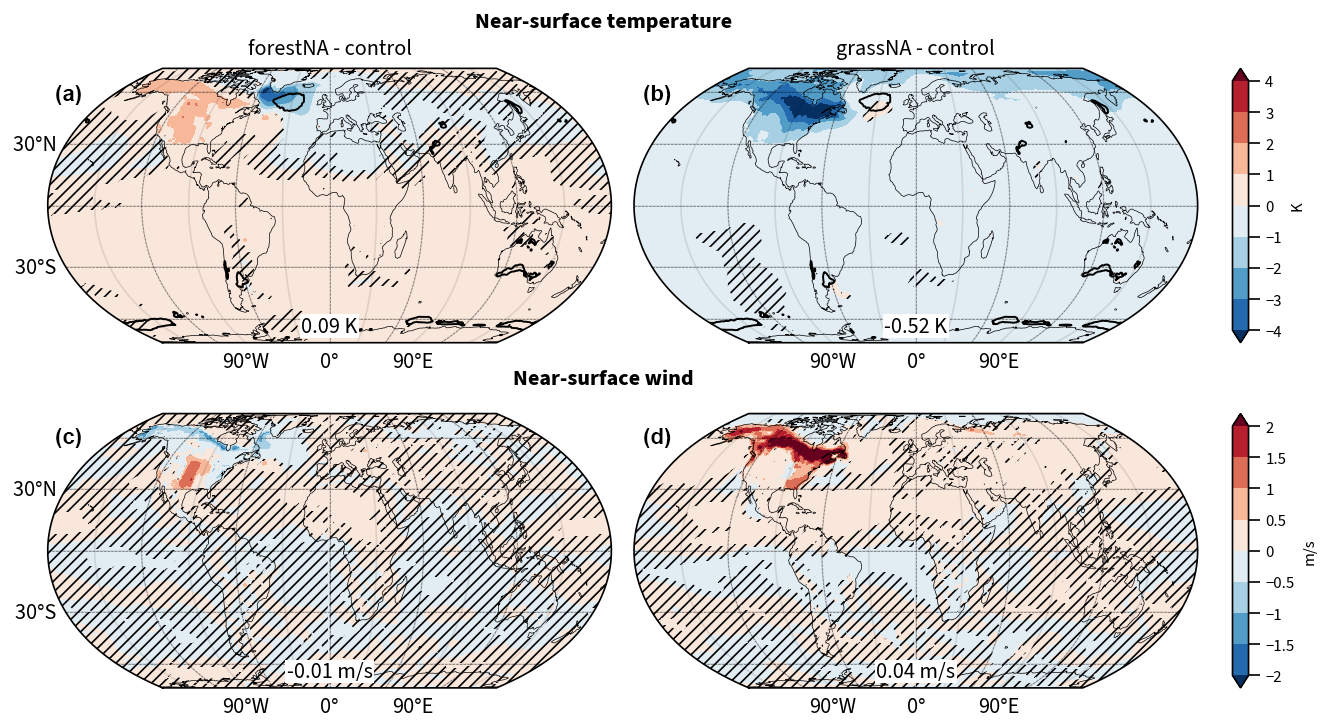
Figure 1 (a, c) Global response of yearly average near-surface temperature (b, d) and near-surface wind to forestation (forestNA–control) and deforestation (grassNA–control) over North America. Shown is the average over the years 50 to 300 of the corresponding simulation relative to the control run. Numbers in boxes indicate globally averaged changes. Hatching indicates statistically insignificant differences. The black contour in panels (a) and (b) denotes the 0 K/century trend in the monthly ERA5 reanalysis near-surface temperature from 1950 to 2023 (Hersbach et al., 2023) to indicate the extent of the historical North Atlantic warming hole.

Naturally, the global mean temperature response is weaker when limiting forest cover changes to North America compared to global forestation (Portmann et al., 2022). In Portmann et al. (2022), global forestation was shown to increase global mean near-surface temperatures by 0.49 K, and deforestation was shown to decrease it by 1.58 K (Fig. B3a, b). Moreover, the temperature response over North American land is also weaker, most likely due to the reduced advection of anomalously warm/cold air from Asia to North America. Meanwhile, the response in the North Atlantic SSTs is remarkably similar. The warming hole in forestNA is of a similar spatial extent and magnitude to the warming hole in response to global forestation. The cooling hole in grassNA is weaker compared to global deforestation but of a similar spatial extent. This shows that forest cover changes over North America alone are sufficient to result in a negative North Atlantic SST anomaly that is similar to global forest cover changes. This points towards an enhanced sensitivity of the North Atlantic Ocean to upstream forest cover changes.

A qualitative comparison of the forestNA warming hole to the historical NAWH found in ERA5 reanalysis data (Hersbach et al., 2020, 2023; black contour in Fig. 1a, b) shows that the NAWH in forestNA is more pronounced in the Labrador Sea instead of having its greatest anomaly in the central North Atlantic. Indeed, the location and spatial extent of the observed warming hole are more similar to that of the cooling hole in grassNA. This is also true in comparison to the projected NAWH at the end of the 21st century under a high-emission scenario (RCP8.5), where the greatest magnitude of the NAWH is shifted to the east of Greenland (Menary and Wood, 2018) instead of the Labrador Sea. This raises the question of why the warming hole in forestNA is shifted into the Labrador Sea compared to the SST anomaly visible in grassNA, as well as historical data and anthropogenic warming projections. This is further explored in Sect. 3.2.

Compared to global forestation and deforestation, near-surface wind speed changes are almost identical over North American land (Fig. B3c, d). Forestation decreases near-surface wind speed in the north, from Alaska to Quebec, by up to 1 m s⁻¹ (Fig. 1c). In central North America, we see a positive wind anomaly, as in the global forestation scenario (Fig. B3c), the cause of which is not entirely clear. Potentially, this very dry region is not sustaining the afforestation and thus simulates less roughness than the vegetation in the control run (most likely crops or grass), which agrees with the absence of significant changes in canopy height in this region (Fig. B1c). Moreover, orographic effects downstream of the Rocky Mountains, in combination with changes in thermally driven circulation, could influence this response. However, the impact of these changes is local, and it is reasonable to assume that this increase in wind speed has only a weak downstream influence on the North Atlantic. It is beyond the scope of this study to investigate this local change in the wind speed. In contrast, deforestation leads to a significant increase in near-surface wind speeds over North America, with the strongest increases located in the northeast (Fig. 1d). Locally, wind speed increase can exceed 2 m s⁻¹. Similarly, over the warming hole region in forestNA, the wind speed decreases, while in grassNA it increases, which is potentially related to the SST anomalies as further discussed in Sect. 3.4.

In this study, AMOC strength is quantified as the maximum of the zonally averaged meridional overturning streamfunction between 20 and 70° N and below 500 m (AMOC index; Liu et al., 2020; Portmann et al., 2022). In grassNA, the AMOC strength increases very rapidly during the first 25 years of the simulation to a peak value of 39 Sv, which is about 11 Sv or 40 % above its long-term median. This large increase in grassNA (compared to the reaction in forestNA) may be attributable to the fact that albedo and temperature changes over land are stronger in grassNA than in forestNA (Figs. B1e and f and 3b) and that the anomalously cold branching point may favour increases in deep convection. Moreover, there might be a positive feedback of warmer and saltier ocean waters and the sensitivity of deep convection to atmospheric forcing, as further explored in Sect. 3.2. While such fast AMOC increases have been found in other studies as well (Haskins et al., 2019; van Westen and Dijkstra, 2023), explaining the initial phase of the AMOC reaction remains a challenge due to many effects overlapping over a very short time period. In forestNA, the AMOC declines in comparison to the control run. This reaction is slower than the one in grassNA and is likely connected to the slowly building sea ice feedback explored in Sect. 3.2. Note, however, that this paper focuses primarily on the mechanisms governing the long-term response of the AMOC. Nevertheless, we want to show the initial response for comparability and possible future studies. In the long-term response, the median AMOC strength declines in forestNA by 12 % or 2.0 Sv to a median of 20.6 Sv, while it increases in grassNA by 20 % or 4.7 to 28.1 Sv (Fig. 2c). In comparison, global forestation weakens AMOC by 22 % in Portmann et al. (2022), and deforestation strengthens it by 49 %. Thus, while we find a warming hole of a similar intensity in forestNA compared to global forestation simulations, the AMOC reduction is less pronounced. This shows that the strength of the warming hole does not depend linearly on the AMOC strength, corroborating the findings from Keil et al. (2020). That the responses of the AMOC and SSTs to forestation and deforestation are non-linear can be linked to a sea ice feedback, as discussed in Sect. 3.2. However, further factors like shortwave cloud feedbacks or the export of water towards higher latitudes might also play a role here (Keil et al., 2020).

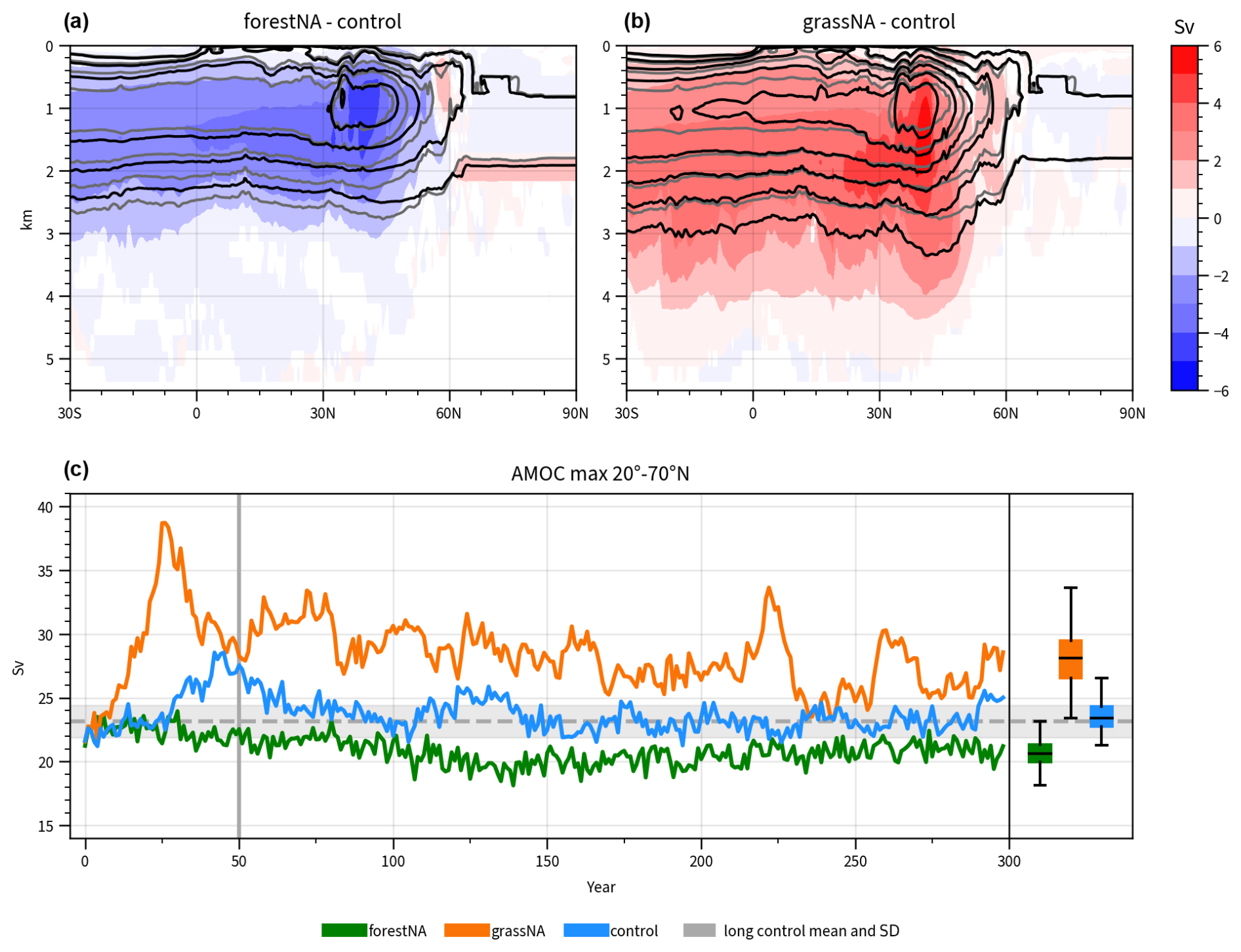
Figure 2 Depth profile of changes in the zonally averaged overturning streamfunction for (a) forestNA and (b) grassNA for the years 50 to 300. Shading represents scenario differences with respect to the control run in steps of 1 Sv, with statistically insignificant changes masked in white. Contours show absolute values in steps of 4 Sv, starting at 4 Sv for forestNA and grassNA in black and in grey for the control run. (c) Time evolution of the AMOC index for forestNA (green), grassNA (orange), and control runs (blue). In grey, the mean and standard deviation of the AMOC index of the second half of the 1000-year-long control run is shown. The box plots summarise the evolution over the years 50 to 300 for forestNA (green; left), grassNA (orange; middle) and control runs (blue; right). Black lines indicate the median, while boxes show the interquartile range. Values outside of 1.5 times the interquartile range are treated as outliers. The vertical grey lines mark the years 50 and 300.

The zonal average of the overturning circulation (i.e. the AMOC streamfunction) decreases in forestNA in almost the entire basin, except for a positive anomaly at 60° N, suggesting a slight poleward shift in the streamfunction (Fig. 2a). Moreover, overturning becomes more shallow. In grassNA, changes are of the opposite sign and stronger compared to forestNA (Fig. 2b). In the height coordinates, the AMOC intensifies and deepens. The maximum anomaly in comparison to the control run is shifted to a greater depth than in forestNA. For forestNA and grassNA, changes in the zonally averaged AMOC are weaker and shallower compared to global forest cover experiments (Portmann et al., 2022). Similar to Portmann et al. (2022), AMOC changes are computed in potential density coordinates (Fig. B2), which, in line with the global simulations, shows that AMOC maxima and their changes occur further poleward. Note that the overshoot of the AMOC index during the first 70 years of the control run relates to model-specific sea ice variability (Danabasoglu et al., 2020a). While the AMOC index of the control run remains within the variability in the last 500 years of the longer control simulation (grey range in Fig. 2) from which it was branched, forestNA and grassNA mostly lie outside that range after year 50. In the context of anthropogenic warming, the annual mean AMOC response to North American forestation is weaker compared to that projected in RCP8.5 global warming scenarios for which Rahmstorf et al. (2015) project a decrease of up to 8 Sv and Liu et al. (2020) a decrease of 10 Sv. When halving the wind stress, Lohmann et al. (2021) find a stronger weakening of the AMOC with similar vertical structure to forestNA, albeit no equatorward shift. Conversely, when doubling the wind stress, they observe a shift in the AMOC to a greater depth (with positive anomalies close to the surface) instead of only a strengthening and deepening as seen in grassNA. The role of wind stress in our simulation is discussed in more detail in Sect. 3.4.

3.2 Mechanisms driving density changes

In this section, we turn to the mechanisms involved in forming the AMOC and SST response through density changes in the ocean waters. Forest cover changes over North America lead to significant changes in albedo (Fig. B1e, f) and temperature (Fig. 1). Changes in albedo are strongest in a narrow band spanning from Alaska (70° N) to Quebec (50° N), with less albedo change north and south of this band in accordance with the changes in canopy height (Fig. B1c, d) and reduced snow albedo feedback further equatorward. Overall, this indicates that there is a very narrow high-latitude band in which the pre-industrial control climate responds strongly to forest cover changes, in agreement with previous studies (Wang et al., 2014; Betts, 2000; Asselin et al., 2022).

To discuss the long-term response of the ocean circulation to the imposed North American forest cover changes, we focus on the winter half-year (December to May, i.e. DJFMAM). First, this choice is justified since the albedo response is the strongest during winter and spring (Fig. B4; Davin et al., 2020; Jiao et al., 2017). This is true especially in the high latitudes due to trees dampening the high albedo of snow. Second, the winter half-year is the period during which the North Atlantic Ocean circulation is most sensitive to atmospheric forcing (Luo et al., 2014; Guo et al., 2024); on the one hand, ocean water cools over the winter and is subsequently the coldest in spring, and on the other hand, sea ice formation during the winter leads to enhanced salt content in spring, making the waters the most dense in this season. Thus, DWF driving the AMOC is most intense in spring (Svingen et al., 2023). This temporal concurrency of the largest impact of vegetation changes and ocean sensitivity likely favours a large response of the ocean to forest cover changes.

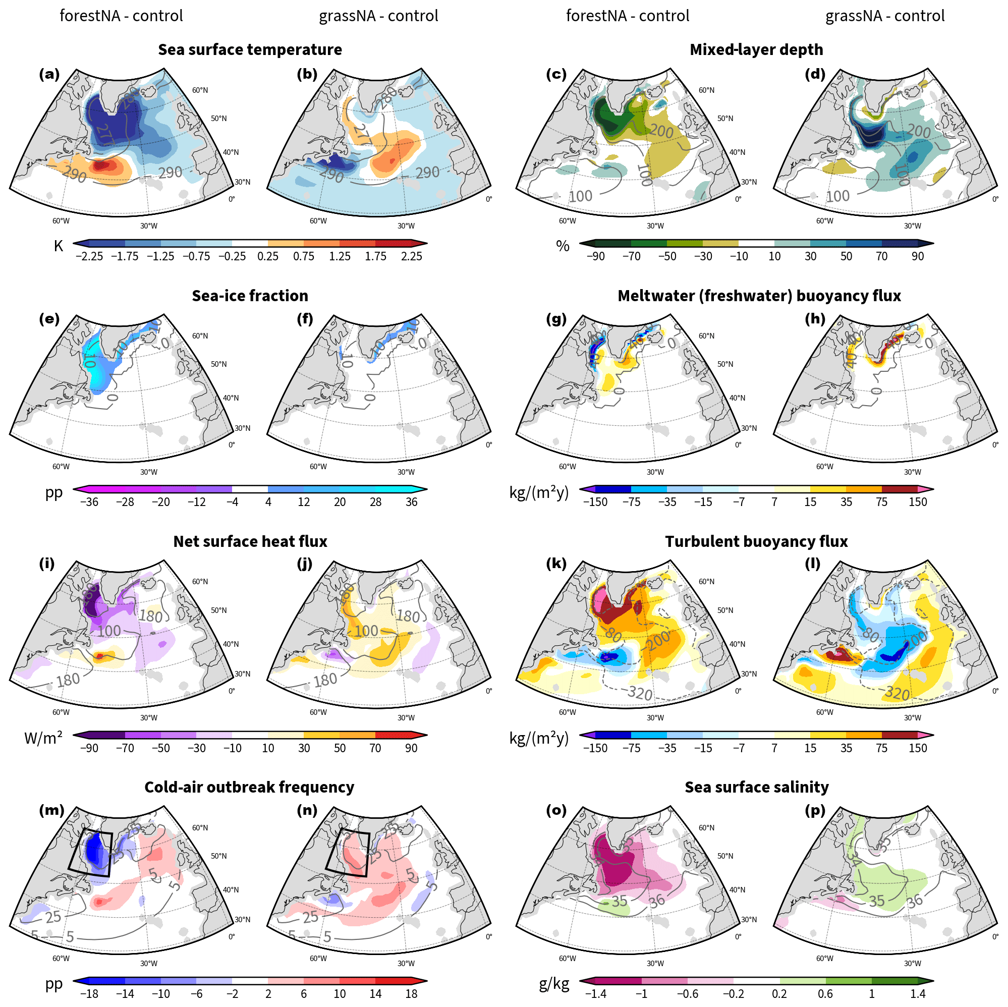
Figure 3 Average changes in the DJFMAM response to forestation (left) and deforestation (right) from the years 50 to 300 of the simulations for (a, b) SSTs; (c, d) changes in mixed-layer depth (MLD) (in %), with absolute values (in m); (e, f) sea ice fraction; (g), (h) meltwater (freshwater) buoyancy flux $B^{{\mathrm{ICE}}_{\mathrm{FW}}}$; (i, j) upward turbulent heat fluxes; (k, l) turbulent buoyancy fluxes B^turb; (m, n) frequency of cold-air outbreaks Δθ>4 K; and (o, p) sea surface salinity. In panels (g), (h), (k), and (l), the positive buoyancy flux anomalies lead to more buoyant surface waters. Grey contours depict absolute values of the control run. Black boxes in panels (m) and (n) signify the Labrador Sea extent used for analyses in Fig. 4 and Sect. 3.3. Note the non-linear colour shading intervals in panels (g), (h), (k), and (l).

The cold SST anomaly in forestNA (Fig. 3a) coincides with the anomaly in the near-surface air temperature in Fig. 1a. It is strongest around the tip of Greenland and covers the whole Labrador Sea west of Greenland. The SST anomaly stretches beyond Iceland in the north and eastward towards the European coast, with a greater intensity towards the southeast. In contrast, the warm SST anomaly in grassNA is strongest in the central North Atlantic, with only a thin branch into the Labrador Sea and Davis Strait (Fig. 3b). Both simulations show strong anomalies of the opposite sign (warm in forestNA and cold in grassNA) east of Nova Scotia. The pattern of a cold temperature anomaly in the North Atlantic with a warm anomaly east of Nova Scotia is also known from observations (Rahmstorf, 2024; Caesar et al., 2018; Zhang and Vallis, 2007) and is part of an SST pattern also referred to as the SST fingerprint in response to AMOC changes.

3.2.1 Mixed-layer depth and sea ice

The Labrador Sea is a region of intensive DWF, which plays a significant role in driving the AMOC and the NAWH (Böning et al., 2023; Garcia-Quintana et al., 2019; Gervais et al., 2018; Kuhlbrodt et al., 2001). A common measure for DWF is the mixed-layer depth (MLD). MLD in this section is defined as the depth of the maximum buoyancy gradient. In forestNA, the negative SST anomaly overlaps with a strong MLD anomaly (Fig. 3c). The reduction in MLD is most pronounced in the Labrador Sea, with extensions east of Greenland and in the southeastern North Atlantic. The negative MLD anomaly is coincides with sea ice growth in the Labrador Sea (Fig. 3c). With DWF mitigated, the AMOC is weakened, and less warm water is imported into the Labrador Sea, facilitating sea ice growth. The advancing sea ice insulates the ocean from the atmosphere, hindering the ocean from losing heat and further inhibiting DWF. This feedback cycle is rather slow and weakens AMOC gradually over time, as seen in Fig. 2c, as sea ice grows slowly over several decades.

In addition to cutting off the heat loss to the atmosphere as the sea ice edge advances, meltwater fluxes shift further toward the open ocean as well (Fig. 3g). Enhanced meltwater fluxes increase the buoyancy of the waters and thus dampen vertical mixing. Buoyancy due to freshwater from meltwater fluxes increases in the Labrador Sea and east of the tip of Greenland. In contrast, buoyancy decreases locally around the control sea ice edge as meltwater and thus fresh water fluxes are missing there. This is why we also see small increases in MLD along the control sea ice edge (Fig. 3e, c).

Sea ice model output confirms that the increase in sea ice is driven by a local SST decrease and not by increased import by wind (not shown). This rules out the hypothesis that wind changes are responsible for the growth of sea ice extent (Schemm, 2018); the net sea ice change by dynamics in the Labrador Sea was even found to decrease in forestNA, despite the larger sea ice extent compared to the control run. Note that due to the anomalously cold waters, Labrador Sea ice melt starts later in the year, and we see the largest freshwater flux shift into summer in forestNA (not shown). However, the increased freshwater buoyancy fluxes from ice melting are largely compensated by the additional insulation of the ocean surface by the ice, where otherwise solar radiation would be warming the upper levels of the ocean and manifesting in a negative heat buoyancy flux anomaly. Attempting to compare these two buoyancy flux components is possibly complicated by cloud responses (Keil et al., 2020).

Similar to forestNA, the SST anomaly overlaps with a change in MLD in grassNA (Fig. 3d). Here, MLD increases over most of the North Atlantic, with the greatest anomalies occurring around the tip of Greenland. The northeastern Atlantic is another location of large MLD changes, albeit of smaller magnitude than in the Labrador Sea. Compared to forestNA, only a thin band of anomalous MLD reaches into Davis Strait in grassNA, and MLD even deepens slightly along the southern and eastern coast of Greenland. This is due to the fact that the cooling of Greenland in grassNA leads to slight increases in sea ice along its coast (Fig. 3f) and increasing freshwater fluxes there (Fig. 3d). This narrows the region of increased MLD to the pattern we see in Fig. 3d and leads to decreased SSTs around the southern and eastern coast of Greenland. However, the increased import of warm water by the AMOC in grassNA prevents sea ice from growing extensively. The fact that the strongest changes in MLD do not overlap as well with changes in SST in grassNA as they do in forestNA is due to sea ice. In forestNA, anomalies in MLD and SST are strongest where sea ice is insulating the ocean. This insulation acts to slow down AMOC, which influences SSTs in the whole of the North Atlantic by reduced warm water import.

We want to point out that the role of sea ice for AMOC decline and the SST anomalies in our forestNA simulation is somewhat different from anthropogenic warming simulations. In forestNA, the warming over land is not strong enough to lead to basin-scale melting of sea ice. Thus, freshwater fluxes are not the main driver of the reduction in MLD and AMOC strength here as they are in several anthropogenic warming simulations (Gervais et al., 2018; Liu et al., 2020) or hosing experiments to investigate AMOC decline (Martin et al., 2022; Jackson et al., 2023). Instead, the changes in buoyancy fluxes in forestNA are dominated by turbulent heat fluxes, and sea ice growth acts as a secondary (positive) feedback. Note that in our simulations, the dynamic time evolution of the Greenland ice sheet is disabled to decrease the complexity of the problem. It is possible that warming from forestation would prompt the Greenland ice sheet to melt and make the North Atlantic waters even more buoyant, thereby accelerating AMOC decline (Martin et al., 2022). Note that sea ice in forestNA only starts to grow after around the year 100 onward (not shown). This supports the idea that the atmosphere is the primary driver of the SST change in forestNA.

Overall, sea ice growth is a key factor in dictating the location, extent, and magnitude of the SST anomalies in the North Atlantic. Anomalous sea ice growth due to a slowdown in AMOC is the reason why the simulated NAWH in forestNA is more intense in the Labrador Sea compared to what is found in reanalysis data, where the warming hole is shifted more into the central North Atlantic (Fig. 1a, b), similar to the cooling hole in grassNA. Moreover, it is likely also the reason why the warming hole in forestNA is of a similar strength to the one found in the global forestation experiment of Portmann et al. (2022) (Fig. B3a). The sea ice response depends heavily on the local cooling close to the North American coast and thus leads to similar sea ice extent (not shown) and surface cooling in both simulations.

Heat fluxes and cold-air outbreaks

Addressing the driving mechanism for the reduced vertical mixing in the DWF regions, we find that turbulent air–sea heat fluxes form the main driver of buoyancy changes (Fig. 3i, j). In forestNA, the turbulent heat fluxes decrease strongly under the sea ice and negative net heat flux anomalies extend into the central North Atlantic. For forestNA and grassNA, changes in turbulent buoyancy fluxes induced by the net surface heat flux changes dominate the anomalies in the total buoyancy fluxes in the whole North Atlantic, except for those in close proximity to the control sea ice edge (Figs. 3k, l, and B5). Consequently, the changes in turbulent buoyancy fluxes are of larger importance than (sea ice) meltwater or other buoyancy fluxes, with the exception of the coastal regions. For both runs, turbulent heat flux anomalies are greatest in the Labrador Sea, with sensible heat fluxes dominating over the latent heat fluxes (not shown).

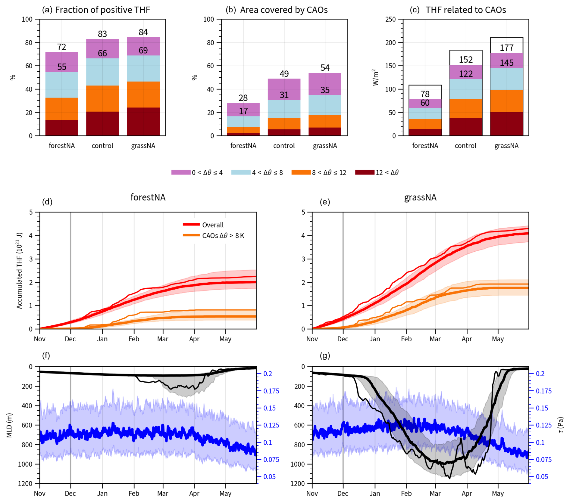
Figure 4 CAO statistics in the Labrador Sea (extent as drawn in Fig. 3m, n) over the years 50 to 300. Panels (a) to (c) are for DJFMAM. (a) The relative fraction of the upward turbulent heat flux (THF) associated with the different CAO categories with respect to all upward THF in the season (i.e. a value of 100 % would indicate that all upwards THF in the Labrador Sea is occurring during CAOs). (b) The area covered by CAOs (equal to the frequency, i.e. fraction of time steps that experience a CAO). (c) The absolute values of the THF associated with CAOs. Categories are according to the potential temperature difference Δθ in colours and transparent if below zero (i.e. the ocean taking up heat from the atmosphere) (c). For a given threshold Δθ, the associated quantity is given by the sum of the categories above the threshold, corresponding to the sum of all the bars underneath and including the respective threshold. Numbers denote the sums for CAOs with strengths greater than Δθ>0 K and Δθ>4 K, respectively. (d, e) Average accumulated THF overall in red and only within in strong CAOs (Δθ>8 K) in orange over November to the end of May for forestNA and grassNA. (f, g) Similarly, the average mixed-layer depth (MLD) is shown in black and wind stress τ in blue. Heavy lines represent the medians and shading the interquartile ranges. In panels (d)–(g), thin lines depict the year 148 as a case study (randomly selected), except for wind stress. Vertical grey lines in panels (d)–(g) mark the start of December.

Several studies in the past have found that air–sea heat fluxes, and subsequently DWF in the North Atlantic, are heavily dependent on CAOs (Svingen et al., 2023; Papritz and Spengler, 2017; Renfrew et al., 2023). Similar to Papritz and Spengler (2017) and Svingen et al. (2023), who focused their studies on the Irminger and Nordic seas and the Greenland Sea, respectively, we find that up to 80 % of heat flux extraction from the Labrador Sea occurs during CAOs (Fig. 4a). Our results show that the number of CAOs with Δθ>4 K in forestNA decreases in the Labrador Sea (Fig. 3m), and so does the total area covered by CAOs (Fig. 4b). Conversely, in grassNA, CAOs increase over the Labrador Sea but also in the central North Atlantic (Fig. 3n). In both cases, changes in strong CAOs (Δθ>8 K) dominate the response in the Labrador Sea, while weaker CAOs respond more strongly over the open ocean (not shown). Subsequently, the heat flux associated with CAOs in forestNA decreases to almost a third of that in grassNA (Fig. 4c), while the fraction of positive heat flux extracted during CAOs compared to times without CAOs only decreases marginally (Fig. 4a). This means that CAOs form the main driver of heat extraction from the ocean in both scenarios. In forestNA, CAOs are becoming less frequent and less strong, mitigating heat transfer to the atmosphere, while the opposite is true for grassNA.

Such a result is also reflected in the evolution of integrated turbulent heat fluxes and MLD during CAOs; changes in MLD overlap well with the integrated ocean-to-atmosphere heat flux associated with strong CAOs (Fig. 4d–g) starting from February onwards. First, weak CAOs continuously extract heat from the ocean from November to December, and no mixed-layer deepening is observed. Only when stronger CAOs extract a lot of heat in short periods of time from January to March will the mixed layer deepen. Starting from around February, strong CAO events push the MLD deeper, while mild CAOs presumably maintain the MLD, as described by Svingen et al. (2023). In forestNA, many of the simulation years do not experience mixed-layer deepening below 100 m at all (Fig. 4f), since extracted heat flux from strong CAOs in spring stagnates (Fig. 4d). It is in agreement with the finding of Holdsworth and Myers (2015) that CAOs play a greater role in warmer years or a generally warmer climate to start DWF. In contrast, the extracted heat content is much higher in grassNA, and so is MLD. These findings further support the hypothesis of a non-linear response of MLD to CAOs and the extracted heat flux.

Note that the average magnitude of wind stress in the Labrador Sea, which could also account for enhanced vertical mixing on the CAO timescale, has a seasonal maximum around February, which is also when the mixed layer deepens most. In line with Fig. 1d, wind stress is slightly larger in grassNA than in forestNA, such that the increased vertical mixing in grassNA compared to forestNA can be partially attributed to faster winds. However, compared to the changes in the accumulated turbulent heat flux, wind stress differences between the simulations are considered small. The effect of wind stress changes on the subpolar gyre are discussed further in Sect. 3.4.

3.2.2 Salinity

In addition to temperature, salinity controls ocean water density. A higher salt content reduces buoyancy, and vice versa. The salinity in the North Atlantic is controlled by freshwater fluxes, evaporation, and import from southerly regions through the ocean circulation (Born et al., 2016; Holdsworth and Myers, 2015). With less salt import, more buoyant waters lead to less DWF and thus reduced AMOC strength. This mechanism is known as the salinity advection feedback (Born et al., 2016). Sea surface salinity (SSS) in forestNA decreases most in the Labrador Sea but also to a large extent in the entire North Atlantic, except for the region of positive temperature change east of Nova Scotia (Fig. 3o).

One could expect that the increased freshwater fluxes in the Labrador Sea away from the control sea ice edge would contribute to a reduced SSS in this region. However, this is not observed in the salinity anomaly, as the pattern is rather distinct from that of the freshwater buoyancy anomaly (Fig. 3g). Similarly, the change in precipitation, evaporation, and runoff buoyancy flux B^PERO is small over the whole North Atlantic and thus negligible for changes in salinity (Fig. B5g). In grassNA, the salinity anomaly is weaker than in forestNA and of a smaller extent. SSS in grassNA increases in the Labrador Sea along the Davis Strait and in the central North Atlantic and also does not display a signature from freshwater forcing. We conclude that the changes in SSS are thus not dominated by changes in freshwater fluxes but instead by the reduced salt advection from southern regions, which is amplified by, and itself amplifying, the AMOC strength reduction through the salinity advection feedback.

Moreover, the salinity anomalies in the northeastern North Atlantic in forestNA and the central North Atlantic are likely the reason for the reduced MLD there, even though we see no strong response of CAOs in this region. The reduced import of salt through reduced AMOC leads to more buoyant waters and thus less DWF. Lohmann et al. (2021) find a salinity decrease with comparable strength in response to the halving of wind stress, leading to a comparable AMOC decline. Similar to their findings, the salinity advection feedback in our study acts to enhance the AMOC changes induced by atmosphere–ocean interactions, i.e. changes in CAOs and associated ocean-to-atmosphere heat fluxes. As a consequence, the salinity advection feedback merely increases the magnitude and large-scale extent of the SST anomalies but is not the leading cause. This is in contrast to studies focusing on meltwater-induced changes in AMOC, where the salt advection feedback is the direct trigger for changes in AMOC and the subsequent SST response (van Westen et al., 2024; van Westen and Dijkstra, 2023).

However, the question arises of how the sensitivity of the ocean to changes in the atmospheric forcing (CAOs and resulting ocean-to-atmosphere heat fluxes) is linked to the ocean salinity. We hypothesise that the salinity state is important for the effect of CAOs. At constant salinity, warmer temperatures lead to a higher thermal expansion coefficient α (Gelderloos et al., 2012; Suckow et al., 1995) and thus a higher sensitivity of the ocean to temperature changes. In addition, the sensitivity to temperature is also enhanced at higher salinity (Suckow et al., 1995). Both combined suggest a higher sensitivity to atmospheric forcing in grassNA, where the North Atlantic is warmer and saltier (Fig. 3b, p). This aligns well with the faster AMOC response to atmospheric forcing at the beginning in grassNA and also the subsequent higher AMOC variability in grassNA (Fig. 2c), given the higher year-to-year variability in atmospheric temperatures (Hogan and Sriver, 2019). The importance of these mechanisms could be investigated by studying different Earth system models featuring different Labrador Sea salinity climatologies or by inducing changes in salinity through modified freshwater forcing in addition to atmospheric perturbations.

3.3 Trajectory analysis

In the previous section, the importance of CAOs for the heat exchange and thereby vertical stratification in the Labrador Sea was identified. However, one objective of this study is to link the changes in atmosphere–ocean interactions to the initial forest cover perturbations. To close this gap, next we investigate backward air parcel trajectories that started during CAOs in the Labrador Sea (region marked by the black boxes in Fig. 3m, n). On the one hand, this allows the identification of the source regions of CAO air masses. On the other hand, by tracing the evolution of several variables along these trajectories, we can disentangle the roles of the changes in sea and air temperatures for heat flux intensities. This helps illustrate the causal pathway from the impacts of forest cover changes on the atmosphere to impacts of the atmosphere on the ocean circulation.

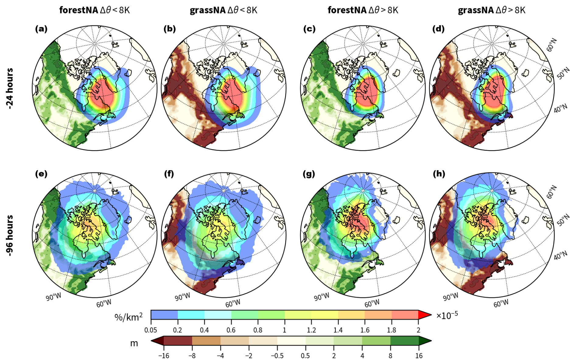
Figure 5 (a–d) Normalised densities of backward trajectories started in the Labrador Sea at −24 and (e–h) −96 h after the starting time (rainbow shading). Trajectories are grouped by the air–sea potential temperature difference Δθ (Sect. 2.5) at the starting time into $\mathrm{0}\le \mathrm{\Delta }\mathit{\theta }\le \mathrm{8}\mathrm{K}$ (a, b, e, f) and Δθ>8 K (c, d, g, h). The densities are normalised as described in Sect. 2.5 and averaged for each time window over DJFMAM of the years 150 to 200. Green and brown shading on land represents the average changes in canopy height (in metres) of the years 50 to 300. Note the non-linear colour scale.

The trajectories are still largely located above the Labrador Sea 24 h before arriving at the target locations, with the highest densities over Davis Strait, Quebec, and east of Greenland (Fig. 5a–d). The trajectories spread further west- and poleward 96 h before reaching their target location, hereafter also referred to as the CAO trajectory source regions (Fig. 5e–h). It is not surprising that the coldest trajectories in the Labrador Sea originate from the climatologically coldest regions like the high Arctic and North American boreal land. These regions are not necessarily regions with forest cover changes. Consequently, we investigate areas within 50 and 90° N and 120 and 60° W that did not experience forest cover changes. Latitudinally averaged vertical profiles show that the air above these grid cells (which are largely overlapping with the trajectory source regions) experiences significant temperature changes (Fig. B7). The warming response in forestNA is stronger in the first 50 years and extends up to 350 hPa, while the cooling response in grassNA is stronger in the long-term response but extends over the entire column in both time periods. The median pressure level of trajectories at −96 h is around 830 hPa. This means that forest cover changes also impact the origin regions of CAO trajectories through remote effects. This is also supported by Guo et al. (2024), who find warming North Atlantic SSTs in response to Eurasian deforestation.

Independently of the scenario, the trajectory densities at −96 h have their maxima around Baffin Island. However, the density of weak CAO trajectories ($\mathrm{0}\le \mathrm{\Delta }\mathit{\theta }\le \mathrm{8}\mathrm{K}$; Fig. 5e, f) in both scenarios is discernibly lower there than the density of strong CAO trajectories (Δθ>8 K; Fig. 5g, h). The weak CAO trajectories are instead spread over a wider area, notably also more towards the east. Moreover, strong CAO trajectories more often come from more poleward regions (150° W) than weak ones. Overall, there is no considerable scenario dependency of the source regions on the coldest air masses arriving at the Labrador Sea. This implies that forest cover changes do not fundamentally change the circulation patterns associated with CAOs.

At the starting time (−0 h), trajectories of weak and strong CAOs show smaller potential temperature differences between the atmosphere and the ocean in forestNA than the ones in grassNA (Fig. 6a). In agreement with this, CAO trajectories in forestNA also see weaker ocean-to-atmosphere heat fluxes (Fig. 6b), as already shown in Sect. 3.2 (Fig. 4c). Note that the probability density of weak CAOs shows several trajectories with Δθ_tra>8 K (Fig. 6a). This comes from the starting height being 100 hPa above the ground (which in the median is around 905 hPa) and not at 850 hPa (which was used for defining CAO masks). While one might expect that the reduced potential temperature difference in forestNA is due to warmer trajectory temperatures, this is not the case. Potential temperatures of strong and weak CAO trajectories at the starting time in forestNA are notably cooler than in grassNA (Fig. 6c). The sea ice and cool SST anomaly in the Labrador Sea in forestNA (Fig. 3a, e) cause the skin temperatures below the trajectories to be considerably cooler than in grassNA (Fig. 6d). Thus, to be part of a CAO, an air parcel in forestNA must be considerably cooler than in grassNA. This is the case 96 h before the trajectories reach the target locations, with weak and strong CAO trajectories still being cooler in forestNA than in grassNA (Fig. 6e). Correspondingly, the total number of trajectories that are cold enough to meet a CAO threshold in forestNA is only about half of the ones in grassNA (Table B1).

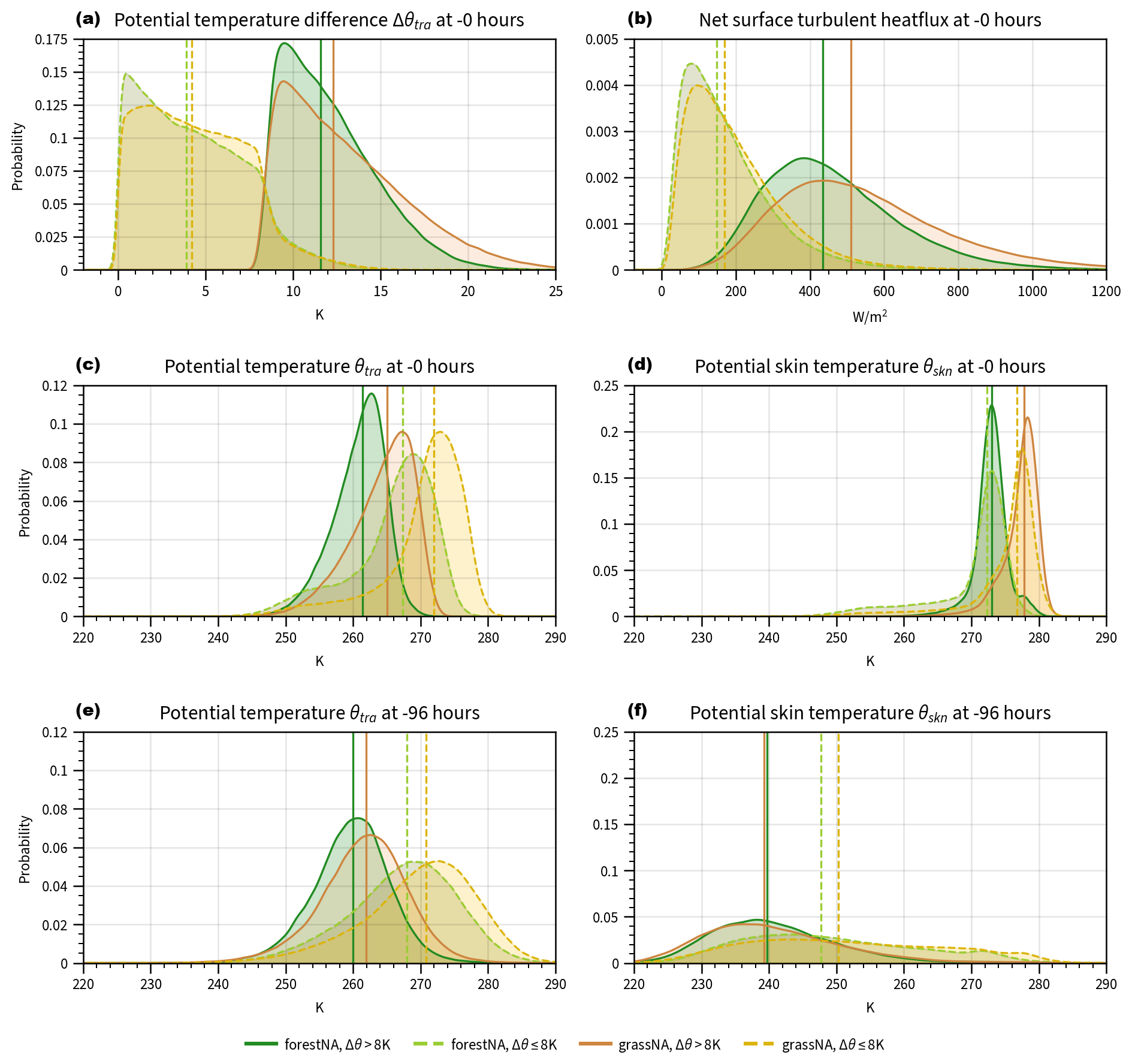
Figure 6 Probability densities of variables traced along the trajectories of the (a) potential temperature difference between trajectory temperature and surface temperature in the target region at −0 h, (b) net turbulent heat flux below the trajectory at −0 h, (c) potential temperature of trajectories at −0 h, (d) potential skin temperature of the surface below the trajectories at −0 h, (e) potential temperature of trajectories in the source region at −96 h, and (f) potential skin temperature of the surface below the trajectories at −96 h. Densities are estimated using kernel density estimation (Parzen, 1962), and medians are marked by vertical lines. Continuous dark lines denote strong CAO trajectories, while dashed light ones mark weak CAO trajectories. The forestNA run is depicted in green and light green, while grassNA is brown and light brown.

Moreover, potential skin temperatures at the starting time in weak CAOs are very similar to the ones in strong CAOs, while the trajectory temperatures differ considerably between the categories. This supports the idea that atmospheric variability is the more important trigger for CAOs than SST variability. One would not expect very low skin temperatures in CAOs, as shown in the tails of weak CAOs (Fig. 6d), yet some weak CAO trajectories might be started over sea ice and very close to land, which leads to very low values in θ_skn. Notably, the skin temperatures below the trajectories in the source region (Fig. 6f) are considerably colder than in the target region (Fig. 6d) because the land is colder than the ocean. While the surface below strong CAO trajectories in the source regions in forestNA is slightly warmer than in grassNA, this is not the case for weak CAO trajectories (Fig. 6f). This is likely due to weak CAO trajectories also originating from regions east of the Labrador Sea, where the influence of the warming hole is strong in forestNA (Figs. 5e and f and 3a).

These results suggest a positive SST and deep-convection feedback mechanism initiated by the forest cover perturbations. In forestNA, a warmer atmosphere makes (strong) CAOs less likely. The ocean response to this is a cooling of the Labrador Sea SSTs (Sect. 3.2) through changes in ocean circulation, which, in turn, makes (strong) CAOs even less likely. In grassNA, the atmospheric response and direction of the feedback are simply reversed. This suggested mechanism of how forest cover changes affect the ocean circulation appears more evidently in grassNA, where the near-surface temperature in the source region of trajectories significantly cools in the long-term response to forest cover removal (Figs. 1b and B7d). In forestNA, the source region of trajectories is not consistently warmer during the years 50–300 but actually slightly cooler over the Arctic Archipelago (Figs. 3a and B7b). We propose that this is a consequence of the feedback itself; i.e. the SST cooling (and related sea ice processes) also cools the adjacent land regions. This is supported by the warming of the atmospheric column over regions without forest cover changes in the trajectory source region during the first 50 years of forestNA (Fig. B7a). In the long-term response, the cooling signal of the NAWH transfers far up into the troposphere, and the warming upstream is mitigated (Fig. B7b).

To further support the idea that warming due to forestation influences CAOs and that this initiates the SST feedback loop, we investigate the distributions of daily minimum near-surface temperatures in the source regions of the CAOs during the years 150 to 200. While the daily minimum near-surface temperature distribution over the considered source region in forestNA is similar to the control run (Fig. B8a), it is shifted to warmer temperatures in grid cells with large forest cover changes (Fig. B8c). Conversely, the distributions in grassNA shift to lower temperatures independently of which regions are considered (Fig. B8b, d). Thus, the coolest temperatures in the source region, which are needed for the formation of strong CAOs, are significantly impacted by forest cover changes in grassNA. In the long-term response in forestNA, the effect of forestation is dampened by the cool anomaly in the Labrador Sea which, in contrast to the abrupt forest cover changes, only establishes after some decades, as also seen in Fig. B7b.

3.4 Changes in wind stress forcing

In this section, we complement the previous buoyancy-focused analyses with a brief assessment of the dynamical influence of wind changes on the subpolar gyre circulation. Forest cover change goes along with a downstream surface wind response over the subpolar North Atlantic (Fig. 1c, d). The forcing of surface wind stress on the ocean circulation has been addressed in several recent studies that discuss North Atlantic surface temperature anomalies (Putrasahan et al., 2019; Hu and Fedorov, 2020; Lohmann et al., 2021; Ghosh et al., 2023), though the interplay between wind stress and buoyancy forcing (and its dependence on model resolution) on subpolar gyres is still the subject of current research (Hogg and Gayen, 2020; Liu et al., 2022; Bhagtani et al., 2023). Given that wind changes have been attributed an important role in ocean circulation changes in the North Atlantic – e.g. through heat transport induced by Ekman flow (Hu and Fedorov, 2020), by shifting the North Atlantic current (Ghosh et al., 2023), or by transporting density anomalies (Kostov et al., 2024) – we want to investigate the connection between surface wind stress and North Atlantic Ocean circulation changes in our simulations as well. We think it is insightful to inspect wind stress changes and its potential effects on the North Atlantic Ocean circulation in more detail, even if it is argued that decadal AMOC variability is closely related to the variability in buoyancy forcing (in CESM2) as also found above (Yeager, 2015).

In an extensive analysis of the NAWH in global warming simulations, Gervais et al. (2018) find a reduction in westerlies over the North Atlantic Ocean, which is qualitatively in line with reduced winds and lower North Atlantic SSTs in our forestNA simulation (Figs. 7a and 1a and c). In contrast, Hu and Fedorov (2020) find stronger westerlies to be associated with a more intense NAWH, which opposes our findings of not only the NAWH being linked to weaker westerlies in forestNA but stronger westerlies occurring together with a cooling hole in grassNA (Figs. 7b, 1b). Similarly, enhanced wind stress in Lohmann et al. (2021) was linked to a strengthened gyre circulation leading to a warming hole – unlike in our grassNA simulation in which a stronger North Atlantic subpolar gyre is found to match a cooling hole (Fig. 7f). Note that while Lohmann et al. (2021) analyse idealised MPI-ESM version 1.2 runs, Gervais et al. (2018) and Hu and Fedorov (2020) investigate CESM1 simulations. In summary, the discrepancy between Hu and Fedorov (2020) and our results suggests that arguments solely based on Ekman-induced heat transport into or out of the NAWH region are too simple.

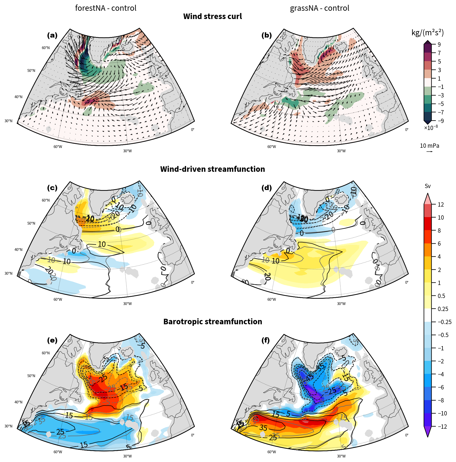
Figure 7 Annually averaged wind curl anomalies from the control run (shading) with wind stress anomalies (arrows) for (a) forestNA and (b) grassNA. A positive wind stress curl anomaly represents a more cyclonic curl. (c, d) Estimated wind-driven streamfunctions of the control run (grey contours), the scenarios (black contours), and the respective anomalies of both scenarios (shading). (e, f) The absolute barotropic streamfunction of the control run (grey contours) and the scenarios (black contours) and anomalies (shading). In panels (c)–(f), a negative streamfunction corresponds to a cyclonic circulation and a negative anomaly in these regions to an intensification of the flow. Please note the non-linear colour scale in panels (c)–(f). Data are taken again from the years 50 to 300.

To assess the contribution of changes in the wind-driven ocean circulation in comparison to the overall barotropic flow, we compare the estimated Sverdrup transport (Eq. 3) against the model output barotropic streamfunction. Here, annual averages are chosen over DJFMAM for comparability with aforementioned studies. Note that changes in wind stress, wind-driven streamfunction, and barotropic streamfunction are slightly stronger during DJFMAM but not qualitatively different (not shown). In forestNA, the anti-cyclonic wind stress curl anomaly around Greenland (Fig. 7a) induces a reduced anticyclonic flow in the Labrador Sea (Fig. 7c). In grassNA, the response to the positive wind stress curl in the Labrador Sea is likewise a decreased streamfunction (enhanced anticyclonic gyre circulation) in this region (Fig. 7d). South of 50° N, a negative wind stress curl anomaly extends across the North Atlantic, with a corresponding positive change in the wind-driven streamfunction.

For forestNA and grassNA, the induced changes in the wind-driven streamfunction (Fig. 7c, d) are, however, rather small compared to changes in overall barotropic streamfunction (Fig. 7e, f). The barotropic gyre circulation is weaker (less cyclonic) in forestNA across the entire North Atlantic and especially at its southern flank, which results in a reduced meridional extent of the flow. However, note that the sign of the streamfunction changes agree north of 45° N, which means that wind changes potentially amplify the density-driven circulation changes. The gyre becomes stronger in grassNA and extends much further south than in the control run. Here, the streamfunction changes feature the same sign in the Labrador Sea and south of 40° N, but the latitude of the sign flip differs by 10°. Given that the estimated changes in the wind-driven streamfunction are small overall compared to the overall barotropic streamfunction anomalies, we conclude that the gyre circulation changes can be largely attributed to density changes as found before in other studies (Liu et al., 2019). A detailed explanation of how winds transport density anomalies in the gyre region (and thereby amplify or dampen the ocean circulation response) (Kostov et al., 2024) is beyond the scope of this study.

The changes in surface wind patterns over the ocean are not uniform across the subpolar North Atlantic but contain patterns that overlap with SST changes (compare Figs. 3a, b to 7a, b around 45° N and between 50 and 30° W). This suggests that the wind response and, subsequently, the effect on the ocean circulation are part of a feedback loop rather than solely a direct response to the forest cover changes upstream. In grassNA, for instance, an increased baroclinicity around 50° N and 40° W might be linked to an enhanced cyclone frequency that footprints in a cyclonic surface wind field anomaly seen around 43° N and 40° W (Gervais et al., 2019). The corresponding positive wind-driven streamfunction aligns with the positive change in the barotropic streamfunction; thus, the induced wind pattern would act as a positive feedback in this case. Similarly, in forestNA, the colder SSTs in the Labrador Sea correspond to a local reduction in baroclinicity, reduced cyclonic winds, and ultimately a reduction in the ocean streamfunctions. In general, however, the overall role of wind in the process chain remains difficult to identify.

Any potential SST–wind feedback loop is likely broken in Lohmann et al. (2021) due to adding a wind stress value from a separate control simulation at each grid cell. This, in addition to other model dependencies, could explain a part of the fundamentally different simulated gyre responses between their and our study. Ruling out the model dependency, the different response in Hu and Fedorov (2020) could be explained by the different model resolution (4° in Hu and Fedorov, 2020, versus 1° in our simulations). Other than that, the opposing results could mean that either buoyancy forcing is the more important driver of North Atlantic Ocean circulation changes (in CESM) or that the gyre circulation is very sensitive to the exact geographical distribution of wind stress changes.

4 Discussion and conclusions

This study illustrates the biogeophysical effects of idealised North American forest cover changes on the North Atlantic Ocean circulation. Foresting North America induces warming on the global scale due to the albedo effect dominating at high latitudes, which is most pronounced over North American land, however, with a cooling anomaly in the subpolar North Atlantic. This is known as the NAWH from other forestation but also global warming experiments (Portmann et al., 2022; Guo et al., 2024; Keil et al., 2020; Gervais et al., 2018). This cold anomaly extends downstream across Europe and Asia, with local cooling in these remote regions reaching up to −1 K. Conversely, in forcing North American vegetation-sustaining areas to be grasslands, global surface temperatures reduce, despite again featuring an anomaly of the opposite sign in the North Atlantic. The effective changes in canopy height from forest cover changes are shown with the resulting changes in SSTs in Fig. 8a for forestNA and Fig. 8b for grassNA. Apart from the NAWH being of comparable magnitude, these changes are generally in line with being weaker than the global-scale equivalents (Portmann et al., 2022). The location and spatial extent of the SST anomalies are similar to global simulations for both experiments. Thus, our findings suggest a high sensitivity of the North Atlantic to upstream forest cover changes. The changes in SSTs are accompanied by AMOC weakening in forestNA and strengthening in grassNA. Yet, the SST response does not depend linearly on AMOC strength confirming findings by Keil et al. (2020).

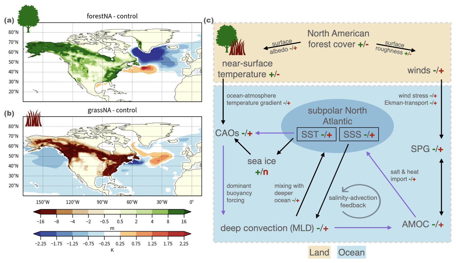
Figure 8 Maps showing changes in canopy height on land and changes in SSTs over the ocean averaged over DJFMAM for the years 50 and 300 for (a) forestNA and (b) grassNA. Note the non-linear colour scale for changes in canopy height.(c) Proposed chain of processes showing how North American forest cover changes impact the North Atlantic Ocean circulation. The “+” and “−” signs indicate increase or decrease in the denoted variable, while “n” indicates no change. Green signs indicate forestNA (always left) and brown grassNA (always right). Arrows marked in purple instead of black denote the positive feedback between CAOs, North Atlantic SSTs, and the AMOC. CAOs are the cold-air outbreaks, MLD is the mixed-layer depth, AMOC is the Atlantic Meridional Overturning Circulation, SPG is the subpolar gyre, SST is the sea surface temperature, and SSS is the sea surface salinity.

The investigated physical processes and identified feedback loops are summarised in Fig. 8c. Through surface albedo and roughness changes, forests directly influence (surface) wind patterns and atmospheric temperatures, which, in turn (in addition to freshwater fluxes), drive the North Atlantic Ocean circulation. In these simulations, ocean-to-atmosphere turbulent heat fluxes were identified as the leading mechanism determining the (long-term) ocean response. The related buoyancy fluxes dominate the response over other buoyancy flux terms (Figs. 3g, h, k, and l and B5). In particular, freshwater fluxes are non-negligible but only make up for a subordinate contribution. Hereby, the extraction of heat from the ocean and thus DWF is mainly governed by strong CAOs (Fig. 4). The frequency of CAOs decreases in forestNA and increases in grassNA (Fig. 3m, n) and so do the corresponding net turbulent heat fluxes (Fig. 4). With reduced ocean-to-atmosphere heat fluxes, the MLD decreases, which results in AMOC weakening in forestNA, and vice versa in grassNA. These changes in AMOC also go hand-in-hand with a reduction in and strengthening of the subpolar gyre circulation in forestNA and grassNA, respectively. The changes in AMOC and the gyre circulation imply changes in heat and salt transport into the subpolar North Atlantic, including the DWF regions. In forestNA, reduced salt import decreases the MLD further (which is not compensated by the density gain due to cooling), and vice versa in grassNA. We find that this salinity advection feedback is subsequently intensifying AMOC and gyre circulation changes (but is not the leading cause thereof, as seen in freshwater-forced simulations used to produce large changes in AMOC; van Westen et al., 2024; van Westen and Dijkstra, 2024). It is also likely that salinity plays a role in the sensitivity of the North Atlantic Ocean to atmospheric forcing, but this mechanism needs further investigation. In addition, (de-)forestation-induced wind stress changes are enhancing the respective subpolar gyre circulation changes but are not strong enough to be identified as the main driver (Lohmann et al., 2021; Liu et al., 2019). Comparing the results with other studies featuring NAWH-like SST anomalies shows that the role of wind stress on the changes in ocean circulation is more complicated than simple Ekman transport arguments can explain.

To bridge the gap between the effect of forest cover changes on the atmosphere and the effect of the atmosphere on the ocean circulation, we performed Lagrangian air parcel analyses. Backward trajectories from CAOs in the Labrador Sea show that the source regions (i.e. the average synoptic situation) do not fundamentally differ between forestNA and grassNA. The upstream source regions are not necessarily regions with the highest forest cover changes but in general the very high latitudes. This suggests that forest cover changes affect Arctic temperatures which contribute to making CAOs in forestNA less frequent and more frequent in grassNA (Fig. 3m, n). This is supported by previous research of Eurasian forest cover experiments which also show similar warming and cooling hole behaviour in Guo et al. (2024). In grassNA, this mechanism appears straightforward. Deforestation leads to a consistent cooling of daily mean and minimum temperatures in the source region (Figs. 3b and B8b). This cooling results in a larger potential temperature difference with the ocean skin temperature, i.e. more CAOs and larger heat fluxes (Fig. 6a, b). In forestNA, the cool anomaly in the Labrador Sea is so strong that air parcels also need to be much cooler to induce a CAO over these colder skin temperatures (Fig. 6c, d). This is a positive feedback in which an initially warmer atmosphere makes CAOs less likely, cooling the ocean via the impacts on the ocean circulation and making CAOs less likely. This feedback is highlighted by purple arrows in Fig. 8c. The resulting cooling in forestNA is so strong that it even cools some of the trajectory source regions (Figs. 1, B8a and c, and B7) but not enough to increase CAO frequencies (Fig. 3m) or ocean-to-atmosphere heat fluxes (Figs. 3i and 6b). Overall, the key mechanism controlling changes in heat loss from the ocean in the Labrador Sea is the change in CAO frequency due to atmospheric temperature changes, which is a direct consequence of forest cover changes.

The cold SST anomaly in the Labrador Sea in forestNA is so strong because sea ice growth acts as a positive feedback by insulating the ocean from heat loss and enhancing AMOC decline. This growth of sea ice is the reason for the fact that the NAWH in forestNA has its greatest intensity in the Labrador Sea, while this is not the case in reanalysis data and future climate simulations (Rahmstorf et al., 2015; He et al., 2022; Gervais et al., 2018). Instead, the location and extent of the warming hole in those cases are similar to the ones of the warm anomaly in grassNA, where there is no such strong anomalous sea ice response. In addition, the strong sea ice response makes the NAWH in forestNA have a similar strength to global forestation experiments (Portmann et al., 2022). The ocean surface simply cannot cool much more than this. Thus, sea ice plays a pivotal role in the response of the North Atlantic Ocean circulation to atmospheric forcing. Notably, the overlapping seasonality of vegetation and MLD sensitivity likely favours a large response to forest cover changes. The high-latitude albedo changes are largest in winter and spring (Fig. B4), as is the positive ocean–atmosphere temperature difference. In conclusion, the North Atlantic Ocean reacts very sensitively and highly non-linearly to upstream forest cover changes. We want to stress that this likely also extends to other cases with upstream temperature forcing. In greenhouse gas forcing simulations, the faster warming of high latitudes known as Arctic amplification resembles the warming response in forestNA (e.g. Rahmstorf, 2024). In principle, we would expect a similar response in CAO frequency and therefore reduced heat loss in regions of DWF. However, the additional freshening by Greenland meltwater might be more important for the salinity advection feedback. Furthermore, changes in wind stress patterns might differ. Nevertheless, the CAO–SST feedback described in this study is likely at play.

This analysis is unique in that it uses 1° spatial- and 6-hourly temporal-resolution fully coupled Earth system model output for analysing the North Atlantic Ocean response to North American forest cover changes, including atmospheric Lagrangian backward trajectories. The main limitation of this study is, however, that only one Earth system model is used. Previous research has shown that the response to vegetation changes varies strongly between different models (De Hertog et al., 2023; Boysen et al., 2020; Davin et al., 2020). Moreover, CESM was shown to model more DWF in the Labrador Sea than other models and consequently react more sensitively to atmospheric forcing in this region (Gervais et al., 2018; Hansen et al., 1999; Liu et al., 2019; Kim et al., 2024). In addition to the model itself, the ocean response also depends on the model resolution (Garcia-Quintana et al., 2019; Jackson et al., 2020; Oldenburg et al., 2022). Future research should incorporate several models, including ensemble simulations for different branching points to exclude the dependency of the response on the initial state of the model. Other than that, a methodological enhancement could be linking events of high vertical mixing to surface heat loss, which would require (sub-)daily surface flux data of the ocean model (to properly account for the insulation effect of sea ice). This could expand on the knowledge about how much the atmosphere contributes to buoyancy changes, for instance, depending on the model resolution (Garcia-Quintana et al., 2019) and the relevance compared to meltwater fluxes. This, in turn, could facilitate the assessment of the relative contribution of CAOs to changes in ocean circulation and the formation of a NAWH in CO₂-forced simulations. The analyses could also be extended to other ocean regions like, for example, the Irminger Sea to study the effects of Greenland tip jets (Pickart et al., 2003).

Last, we want to point out that the setup of our simulations is idealised as it features unrealistically extreme forest cover changes for the sake of identifying the mechanisms controlling the response to forest cover changes in the climate system. Further research is needed to learn about reactions of the ocean and atmosphere circulation to more realistic forest cover changes, for example, in Mo et al. (2023) and how the biogeophysical effects interact with biogeochemical ones, similar to Bala et al. (2007). Simulations from several models, which possibly include different greenhouse gas forcings, would yield more insight into the governing mechanisms in other setups. Our results suggest that forest cover changes upstream in the North Atlantic Ocean can have a great impact on the global climate and should be managed carefully in the future. Reducing carbon emission and halting tropical deforestation are widely accepted as primary goals for decision-makers, while land management can be a powerful local climate change mitigation strategy but has to take remote effects into account (Jayakrishnan and Bala, 2023).

Appendix A: Computation of individual buoyancy flux components

A1 Computation of individual buoyancy flux components

The following are the equations used to compute the individual buoyancy flux components, following Gill (1982):

$$\begin{array}{}\text{(A1)}& {\displaystyle }{B}^{\mathrm{rad}}={\displaystyle \frac{\mathit{\alpha }}{c_p}}\cdot \left(\mathrm{SHF}\mathit{\_}\mathrm{QSW}+\mathrm{LWDN}\mathit{\_}F+\mathrm{LWUP}\mathit{\_}\mathrm{F}\right),\text{(A2)}& {\displaystyle }{B}^{\mathrm{turb}}={\displaystyle \frac{\mathit{\alpha }}{c_p}}\cdot \left(\mathrm{SENH}\mathit{\_}\mathrm{F}+L_v{\mathit{\rho }}_{\mathrm{F}}\cdot \mathrm{EVAP}\mathit{\_}\mathrm{F}\right),\text{(A3)}& {\displaystyle }{B}^{\mathrm{PERO}}=\mathit{\beta }{\mathit{\rho }}_{\mathrm{S}}S\cdot \left(\mathrm{PREC}\mathit{\_}\mathrm{F}+\mathrm{EVAP}\mathit{\_}\mathrm{F}+\mathrm{ROFF}\mathit{\_}\mathrm{F}\right),\text{(A4)}& {\displaystyle }{B}^{{\mathrm{ICE}}_{\mathrm{FW}}}=\mathit{\beta }{\mathit{\rho }}_{\mathrm{S}}S\cdot \left(\mathrm{IOFF}\mathit{\_}\mathrm{F}+\mathrm{MELT}\mathit{\_}\mathrm{F}\right),\text{(A5)}& {\displaystyle }\begin{array}{rl}{B}^{{\mathrm{melt}}_H}& ={\displaystyle \frac{\mathit{\alpha }}{c_p}}\cdot \left(\mathrm{QFLUX}+\mathrm{MELTH}\mathit{\_}F\right)-{\displaystyle \frac{\mathit{\alpha }{L}_f{\mathit{\rho }}_{\mathrm{F}}}{c_p}}\\ & \cdot \left(\mathrm{IOFF}\mathit{\_}\mathrm{F}-\mathrm{SNOW}\mathit{\_}\mathrm{F}\right),\end{array}\end{array}$$

with α as the thermal expansion coefficient, β as the haline contraction coefficient, and other abbreviations of the model variables as found in Table A1.

Table A1 List of CESM output variables used for the buoyancy flux decomposition. Water fluxes are given in kg m⁻² s⁻¹ and heat fluxes in W m⁻².

Appendix B: Additional material

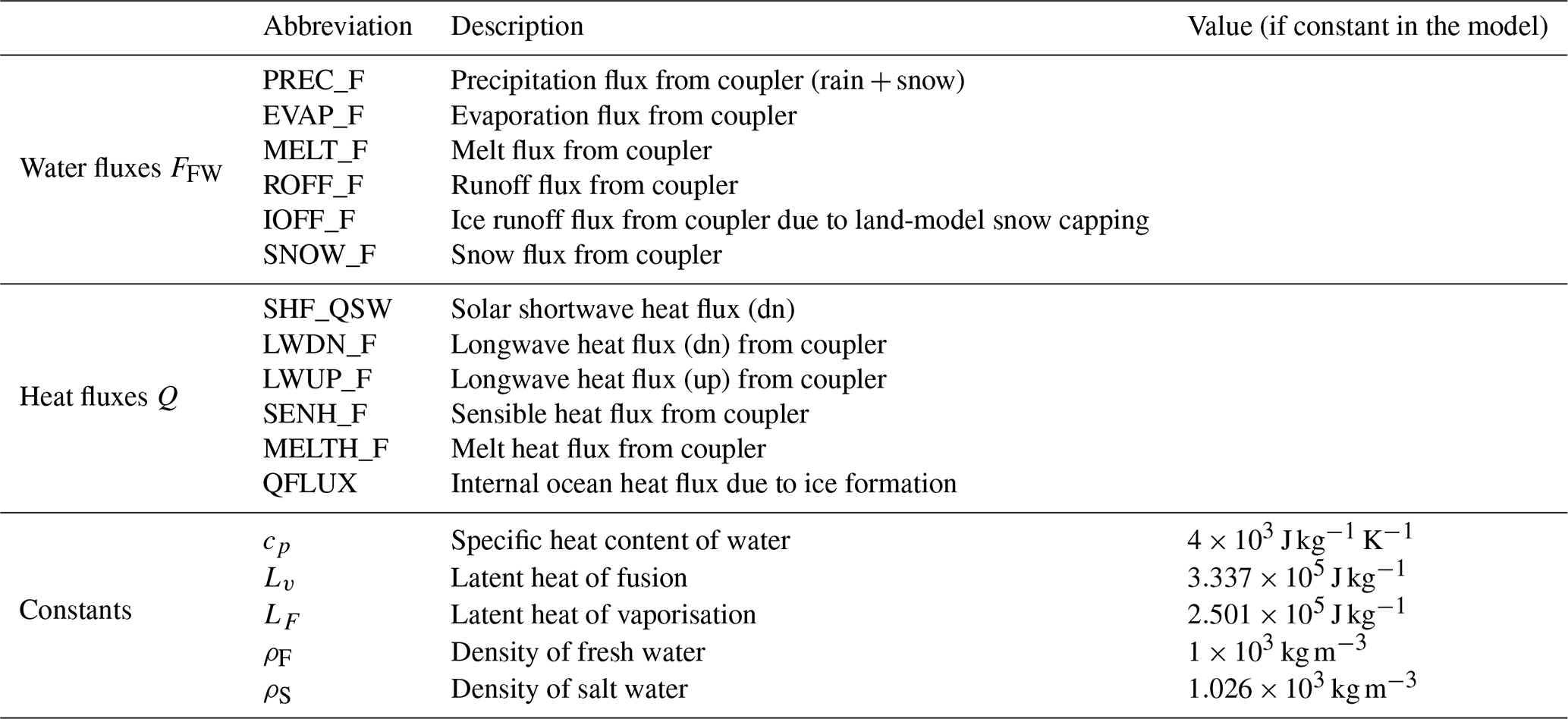
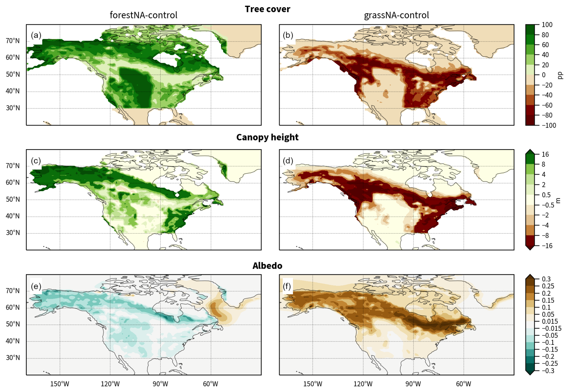
Figure B1 (a, b) Changes in forest cover in percent point (pp), (c, d) yearly average changes in top canopy height (in metres) from the years 50 to 300 (note the non-linear colour scale), and (e, f) yearly average changes in surface albedo from the years 50 to 300 for forestNA (a, c, e) and grassNA (b, d, f) compared to the control run.

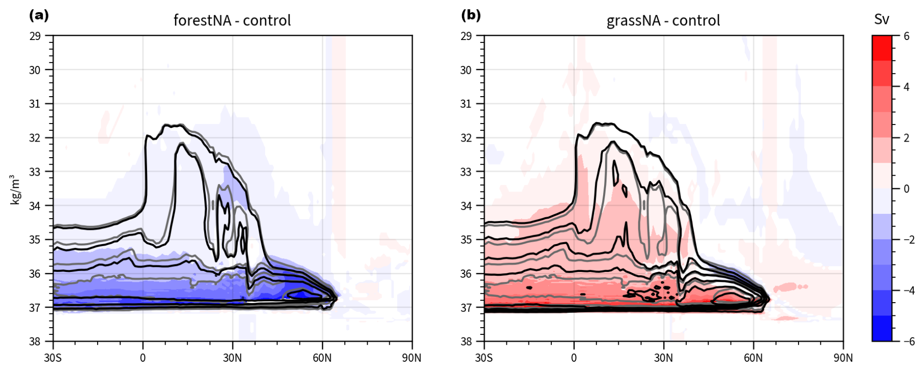
Figure B2 Changes in AMOC in potential density coordinates (a) between forestNA and control runs and (b) between grassNA and control runs (shading), with statistically insignificant changes masked in white. As seen in Fig. 2, the black contours denote the absolute values of the corresponding perturbation scenario, while grey contours refer to the control run.

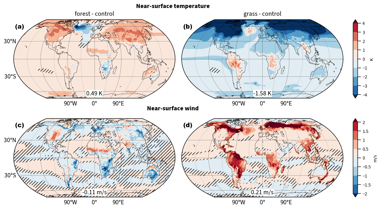
Figure B3 (a, c) Global response of yearly average near-surface temperature and (b, d) near-surface wind to global forestation (forest–control) and deforestation (grass–control) adapted from Portmann et al. (2022). Also shown is the average over the years 50 to 300 for the corresponding simulation relative to the control run. Numbers in boxes indicate globally averaged changes. Hatching indicates statistically insignificant differences.

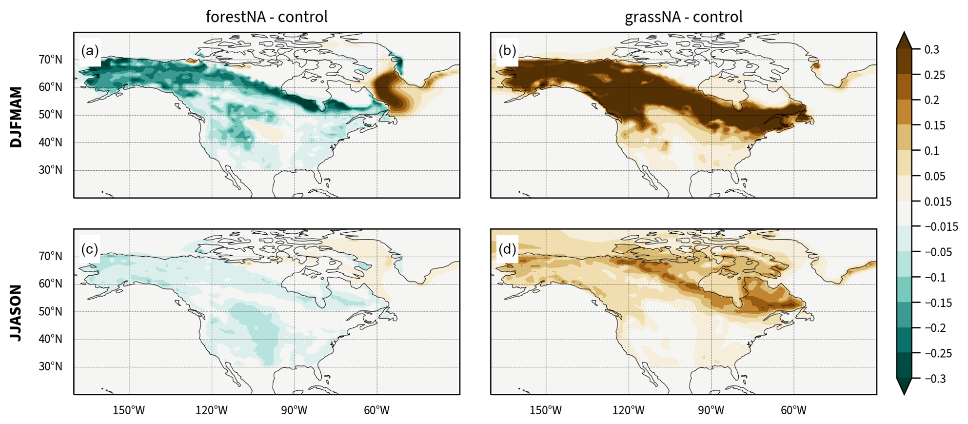
Figure B4 Map of the seasonal average surface albedo response from the years 50 to 300 for forestNA (a, c) and grassNA (b, d) for (a, b) DJFMAM and (c, b) June to November (JJASON).

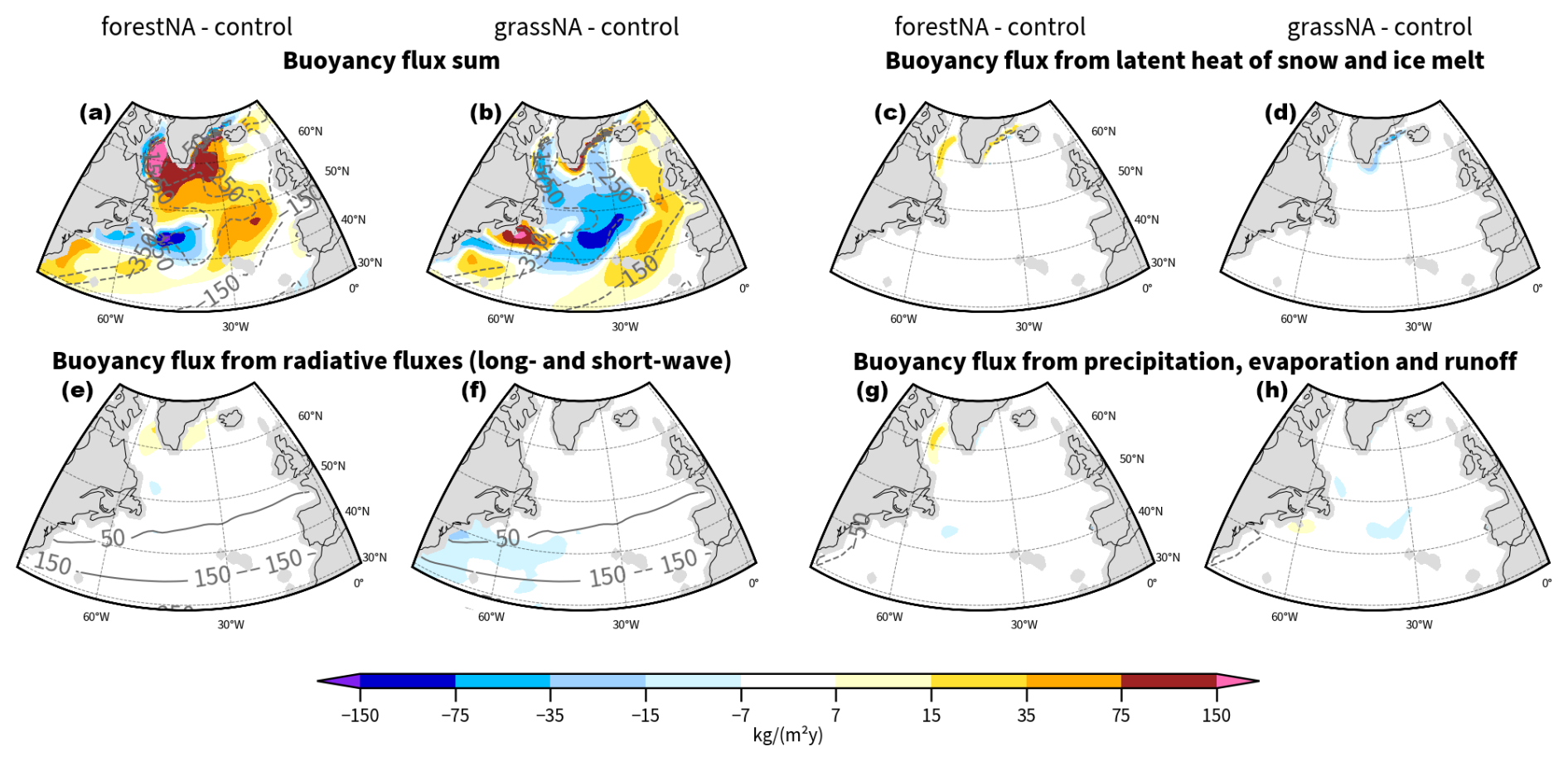
Figure B5 Remaining buoyancy flux components not shown in the main text during DJFMAM. (a, b) Sum of all buoyancy flux terms B. (c, d) Melt heat buoyancy fluxes $B^{{\mathrm{melt}}_H}$. (e, f) Radiation-related buoyancy fluxes B^rad. (g, h) Precipitation, evaporation, and runoff buoyancy fluxes B^PERO. Note the non-linear colour shading.

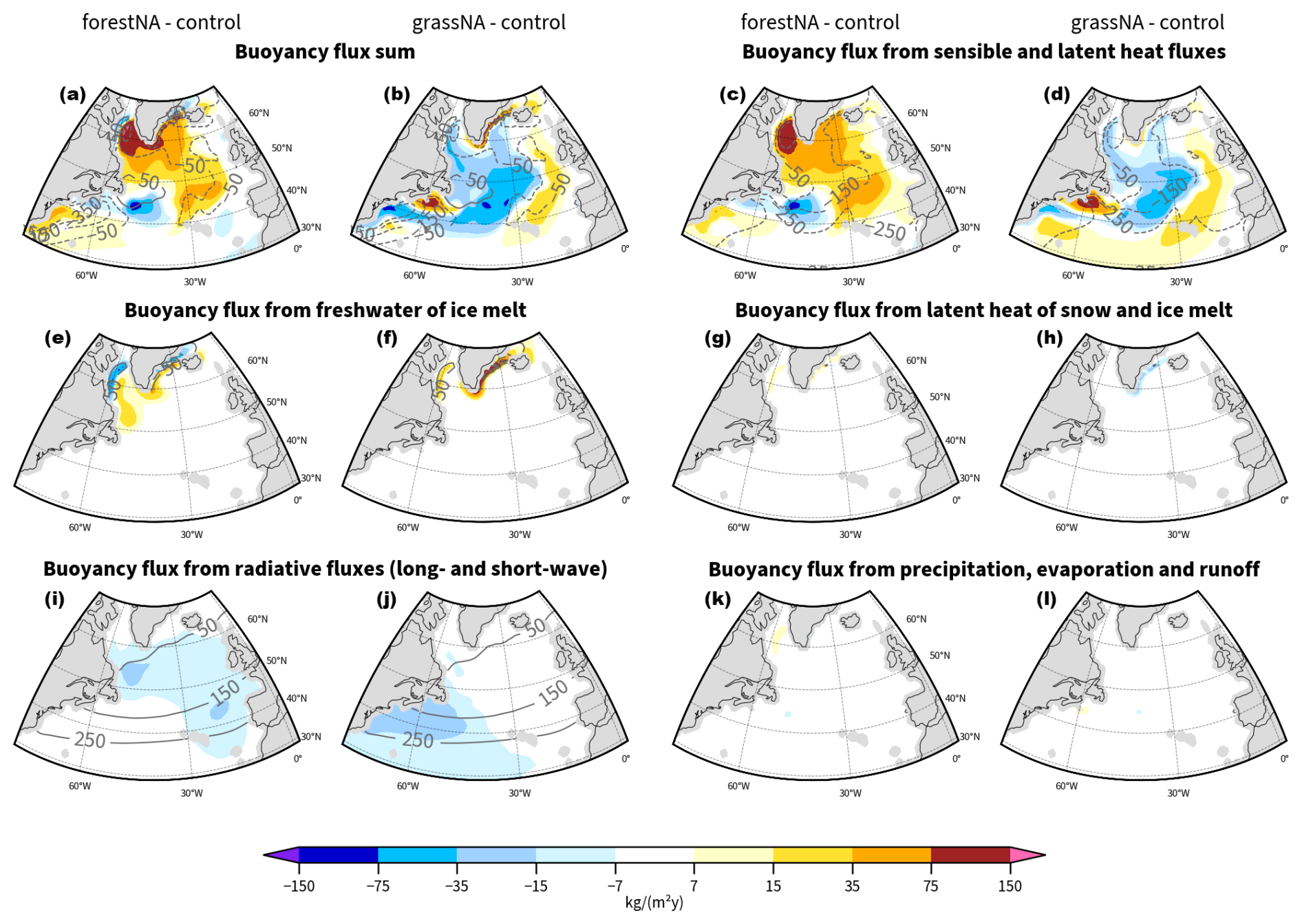
Figure B6 Differences in yearly averaged buoyancy fluxes between forestNA and the control run and grassNA and the control run, respectively. (a, b) Sum of all buoyancy flux terms B. (c, d) Buoyancy fluxes associated with turbulent heat fluxes B^turb. (e, f) Meltwater buoyancy fluxes $B^{IC{E}_{\mathrm{FW}}}$. (g, h) Melt heat buoyancy fluxes $B^{mel{t}_H}$. (i), (j) Radiation-related buoyancy fluxes B^rad. (k, l) Precipitation, evaporation, and runoff buoyancy fluxes. Grey contours show control values. Note the non-linear colour shading.

Table B1 Absolute number of backward trajectories started in CAOs in the Labrador Sea from year 150 to 200 in DJFMAM.

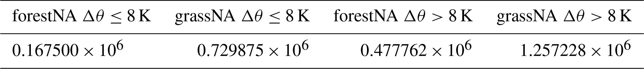
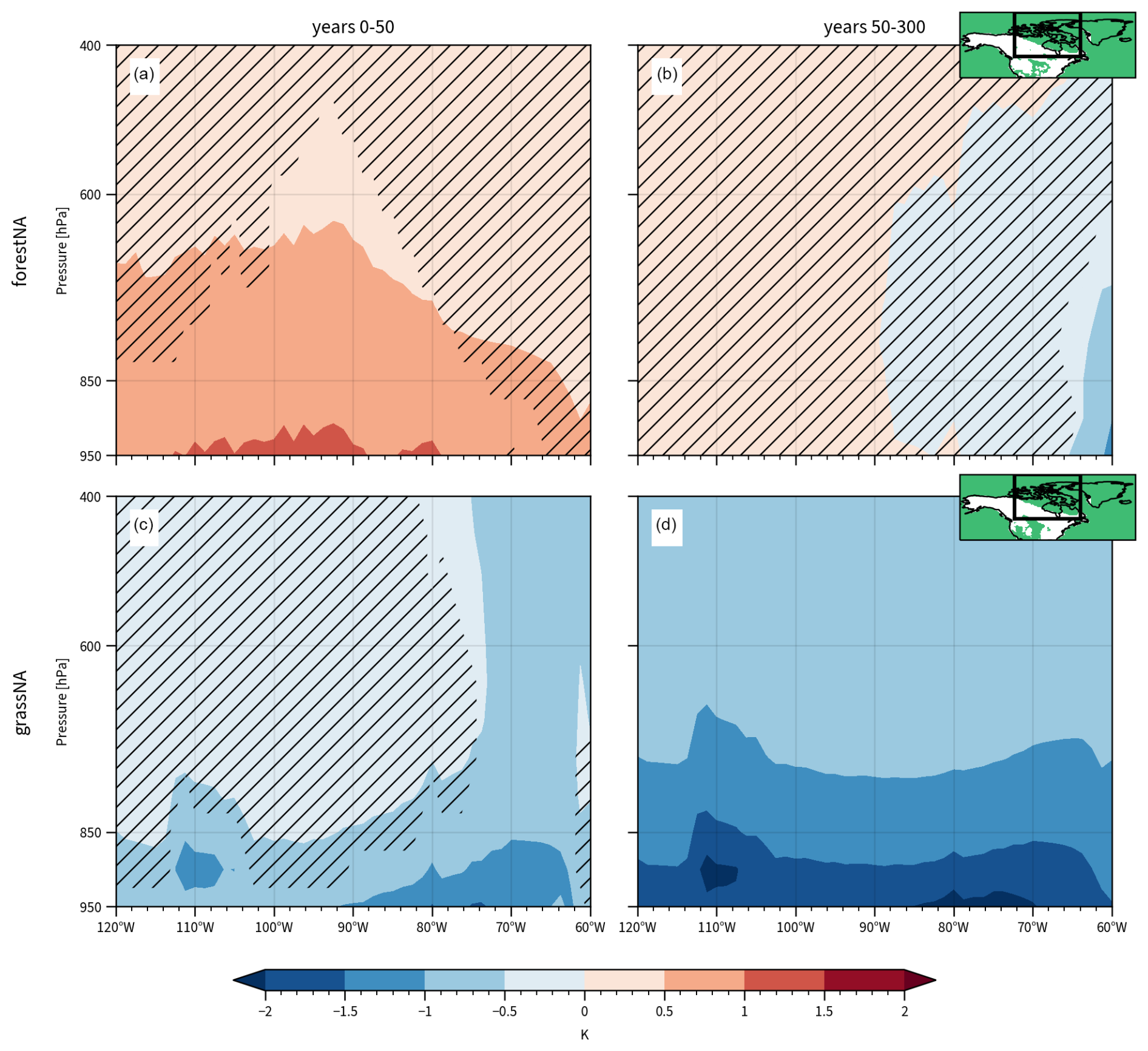
Figure B7 Differences in DJFMAM temperature at pressure levels between 120 to 60° W and averaged over latitudes between 50 and 90° N. Panels (a) and (b) show differences between forestNA and control runs, while panels (c) and (d) show grassNA minus control runs. The left panels are averaged over the years 0 to 49 and right panels over the years 50 to 300. Vertical columns spanning all pressure levels above grid cells with absolute forest cover changes ≤0.5 m were excluded. Insets in panels (b) and (d) show the area (black box) over which the latitudinal mean is taken for forestNA and grassNA, respectively. Excluded grid cells are shown in white and included ones in green. Hatching shows statistical insignificance (same testing procedure as for Fig. 3).

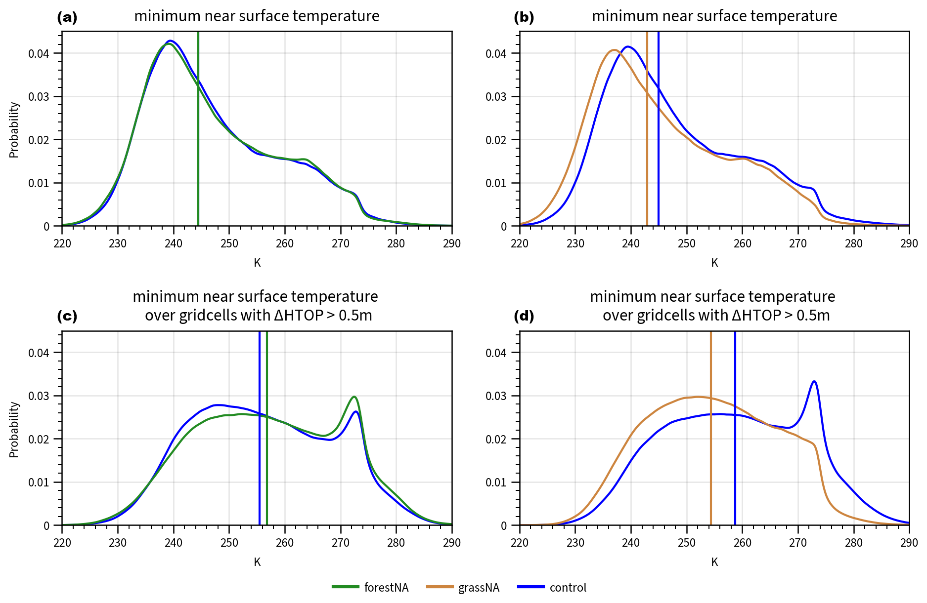
Figure B8 Probability densities of daily minimum near-surface temperature of grid cells masked with trajectory densities $>\mathrm{0.05}\times {\mathrm{10}}^{-\mathrm{5}}$ % m⁻² for DJFMAM in the years 150 to 200 for (a) forestNA (green) and (b) grassNA (brown) and only including grid cells with changes in canopy height > 0.5 m for (c) forestNA and (d) grassNA in comparison to the control run (blue). Probabilities are estimated using kernel density estimation (Parzen, 1962).