Freshwater input from glacier melt outside Greenland alters modeled northern high-latitude ocean circulation

As anthropogenic climate change depletes Earth's ice reservoirs, large amounts of fresh water are released into the ocean. Since the ocean has a major influence on Earth's climate, understanding how the ocean changes in response to an increased freshwater input is crucial for understanding ongoing shifts in the climate system. Moreover, to comprehend the evolution of ice–ocean interactions, it is important to investigate if and how changes in the ocean might affect marine-terminating glaciers' stability. Though most attention in this context has been on freshwater input from Greenland, the other Northern Hemisphere glacierized regions are losing ice mass at a combined rate roughly half that of Greenland and should not be neglected. In order to get a first estimate of how glacier mass loss around the Arctic affects the ocean and how potential changes in the ocean circulation might affect marine-terminating glaciers, we conduct one-way coupled experiments with an ocean general circulation model (NEMO-ANHA4) and a glacier evolution model (Open Global Glacier Model; OGGM) for the years 2010 to 2019. We find an increase in the heat content of Baffin Bay due to an enhanced gyre circulation that leads to an increased heat transport through Davis Strait. We also find changes in the subpolar gyre's structure: an increase in density and a decrease in sea surface height in the eastern part and vice versa in the western part. Additionally, we find a decreased heat transport into the Barents Sea due to increased freshwater input from Svalbard and the Russian Arctic. The rerouting of Atlantic water from the Barents Sea Opening through Fram Strait leads to an increased heat transport into the Arctic Ocean and a decrease in sea ice thickness in the Fram Strait area.

1 Introduction

The recent accumulation of heat in Earth's atmosphere and ocean due to anthropogenic climate change is diminishing the frozen water reservoirs on the planet, causing the release of large amounts of fresh water (Slater et al., 2021). Melting of Earth's glaciers is impacting regional hydrology and increasing global mean sea level (Huss and Hock, 2018; Frederikse et al., 2020). Moreover, such an additional freshwater input to the ocean changes its surface density and thus has the potential to change the ocean circulation on scales ranging from individual fjords (Bartholomaus et al., 2016) to the Atlantic Meridional Overturning Circulation (AMOC; Hu et al., 2011; Frajka-Williams et al., 2016), which is an important component of the global climate system. While there have been numerous studies on changes in the AMOC's strength and a potential influence of recently increased freshwater influx and ocean warming, it is disputed whether the AMOC has already been forced out of its natural variability envelope (Jackson et al., 2022; Latif et al., 2022; Caesar et al., 2021; Fu et al., 2020; Böning et al., 2016). Concerning the regional impact of enhanced Greenland ice sheet (GrIS) freshwater runoff on ocean circulation, Castro de la Guardia et al. (2015) found significant changes in Baffin Bay in a numerical ocean circulation model. These changes entailed an increasing heat content in Baffin Bay with increasing (idealized) freshwater input along Greenland's west coast. This is a potential positive feedback, which could lead to larger heat transports towards marine-terminating glacier fronts. Anthropogenic climate change causes the ocean to take up vast amounts of heat (von Schuckmann et al., 2020). This increase in ocean temperature, in combination with potential changes in ocean circulation, increases submarine melt of marine-terminating glaciers, destabilizing their fronts and inducing further retreat and mass loss (Wood et al., 2021, 2018). Such interactions between changes in ice bodies and the ocean have importance not only for contemporary changes in the Earth system, but also on timescales encompassing glacial cycles (Alvarez-Solas et al., 2013; Rainsley et al., 2018). This underscores the importance of knowledge about the coupled ice–ocean system for understanding past and ongoing changes in the Earth system and for projecting future changes. While there has been previous research on the impact of Greenland melt on modeled ocean properties, mostly focusing on the AMOC, they have either added an idealized high “worst-case scenario” (∼0.1 Sv; e.g., Jackson et al., 2023; Weijer et al., 2012; Castro de la Guardia et al., 2015; Swingedouw et al., 2013) or realistic historical (∼0.01 Sv; e.g., Martin et al., 2022; Martin and Biastoch, 2023; Schiller-Weiss et al., 2024) freshwater flux from Greenland only, or they did not disentangle the impact of the freshwater flux from Greenland and from the glaciers in regions surrounding it (e.g., Devilliers et al., 2021; Swingedouw et al., 2022; Devilliers et al., 2024). Since climate models used for decadal or centennial projections mostly do not include future GrIS melt (Swingedouw et al., 2022), the influence of GrIS melt on future climate model projections has also been studied (e.g., Jungclaus et al., 2006; Swingedouw et al., 2015; Saenko et al., 2017).

Although the most attention in the context of ice–ocean interactions has been on the GrIS, as it is the largest land-ice reservoir in the Northern Hemisphere, there are also other places experiencing glacier mass loss and hence releasing fresh water into the ocean. Around the high-latitude (North Atlantic and Arctic) ocean, such places are the Canadian Arctic Archipelago (CAA), Svalbard, Iceland, and the Russian Arctic. Since ice loss in these places combined is roughly half that of the GrIS over 2010–2019 (∼125 Gt a⁻¹; see, e.g., Hugonnet et al., 2021; Zemp et al., 2019; Slater et al., 2021), it is worth investigating whether increased freshwater input at the coasts of the aforementioned regions due to glacial melt affects the high-latitude ocean circulation, as such changes might also impact marine ecosystems (Timmermans and Marshall, 2020; Hátún et al., 2009; Wassmann et al., 2011; Greene et al., 2008).

Figure 1 charts the main features of the ocean surface currents in the northern Atlantic and the gateways between the Atlantic and Arctic Ocean. Atlantic water masses (red) are characterized as warmer and more saline compared to the Arctic water (blue). Atlantic water is transported to the north, via the North Atlantic Current, by a complex interplay of the mainly wind-driven subtropical and subpolar gyres and the density-driven AMOC. The subpolar gyre (SPG) is the circulation pattern around the Labrador Sea and the Irminger Sea, which transports Atlantic water branching off to the west in the Irminger Sea to the Labrador Sea and into Baffin Bay via the West Greenland Current. The Labrador Sea also is a location of importance for the AMOC, as deep convection takes place there (Broecker, 1997; Yeager et al., 2021), although this view was recently challenged (Lozier et al., 2019). Warm Atlantic water mainly enters the Arctic Ocean through Fram Strait as well as through the Barents Sea, while Arctic water mainly enters the Atlantic Ocean through the CAA and Fram Strait (Lien et al., 2013; Myers et al., 2021; Rudels et al., 2005). Arctic water is transported further to the south mainly by the Labrador Current.

The amount of ice that is removed from glaciers (outside the GrIS) by submarine melt is essentially unknown. Submarine melt remains elusive, since it is complex to measure directly and observations hence remain sparse (Sutherland et al., 2019). Attempts to quantify it therefore mostly rely on high-resolution (∼1 m grid spacing close to the ice front) ocean circulation models employing a parameterization of ice–ocean heat transfer related to oceanic properties at the glacier front (Jenkins et al., 2001; Holland et al., 2008; Xu et al., 2013). As this is computationally costly and can only be applied to individual glaciers, a further step in trying to generalize such modeling results to different glaciers was to employ empirical power laws to describe the relationship between submarine melt and ocean properties as well as subglacial discharge (Xu et al., 2013; Rignot et al., 2016; Wood et al., 2021). We make use of such a power-law parameterization in our attempt to quantify submarine melt of marine-terminating glaciers outside the GrIS.

To tackle the issue of ice–ocean interactions outside the GrIS, we one-way-couple the Nucleus for European Modelling of the Ocean (NEMO) model and the Open Global Glacier Model (OGGM) for the years 2010–2019. We run both models twice in order to investigate potential coupling effects. In one NEMO experiment, we use glacial surface mass loss and frontal ablation derived from OGGM as additional liquid freshwater and iceberg input to NEMO, while we omit this additional freshwater forcing in the second NEMO run. Next, we use the two different NEMO runs' output variables as forcing of the submarine melt parameterization newly implemented in OGGM (see Sect. 2.3.3). We then explore the differences in results obtained from the two different NEMO and OGGM experiments. Through this we aim to obtain a first-order estimate of the effect ice–ocean coupling outside Greenland has on ocean properties as well as on marine-terminating glacier mass loss. Finally, we discuss future avenues for research on this topic, as our rather simple approach warrants further work more closely examining the mechanisms proposed in this work.

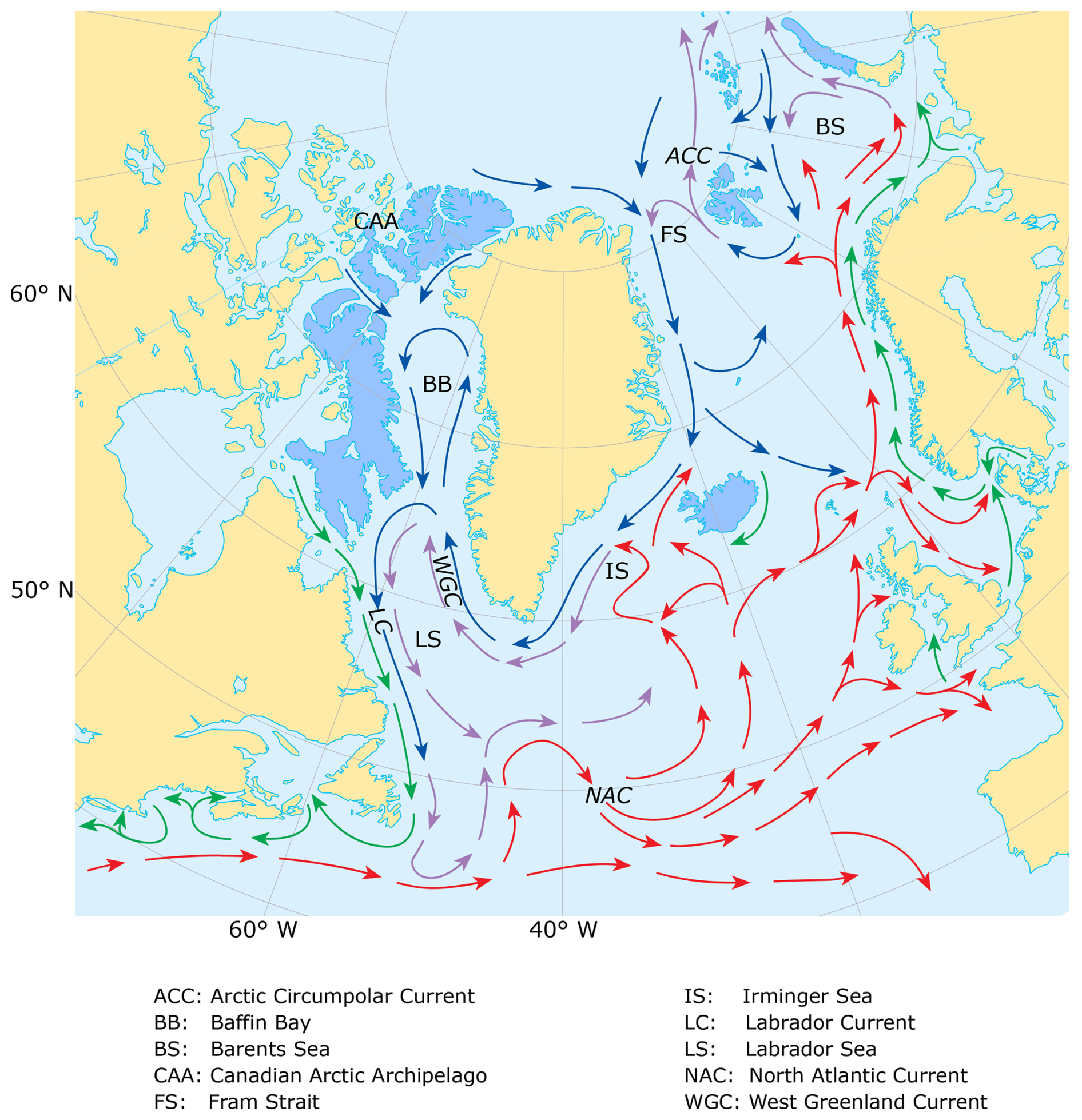
Figure 1 Schematic of the main surface currents in the North Atlantic Ocean. Red and blue arrows indicate Atlantic and Arctic water, and purple arrows show a mixture of both water masses. Green arrows indicate coastal water masses. Blue colored land areas indicate regions that contain glaciers outside of Greenland; see Figs. 11 and 2 for the actual glacier outlines. Italic acronyms represent ocean current names, while the others represent location names.

2 Data and methods

2.1 Ocean model

Our numerical experiments were conducted with NEMO v3.6 (Madec et al., 2017), which is coupled to a sea ice model (Louvain-la-Neuve Sea Ice Model 2; Bouillon et al., 2009). The configuration we use covers the Arctic and Northern Hemisphere Atlantic and has open boundaries at 20° S in the Atlantic Ocean as well as at the Bering Strait. The average horizontal resolution of the model is $\mathrm{1}/\mathrm{4}$°, and it has 50 vertical levels (Arctic and Northern Hemisphere Atlantic (ANHA4) configuration; see Fig. A1). For boundary and initial ocean conditions we use the Global Ocean ReanalYsis and Simulations data (GLORYS2v3; Masina et al., 2017) and for atmospheric forcing the Canadian Meteorological Center's reforecasts (CGRF; Smith et al., 2014). CGRF provides hourly fields of wind, air temperature and humidity, radiation fluxes, and total precipitation with a horizontal resolution of 33 km, which are linearly interpolated onto the NEMO-ANHA4 grid. The Lagrangian iceberg module implemented in NEMO is described by Marsh et al. (2015) and was further developed by Marson et al. (2018). The baseline continental runoff data (outside Greenland) for our runs were obtained by linearly interpolating the data provided by Dai et al. (2009) on a 1×1° grid to the NEMO-ANHA4 grid.

The Dai et al. (2009) data do not cover our model period from 2010 to 2019; we therefore applied the 1997 to 2007 monthly average baseline runoff. Note that the Dai et al. (2009) data do not explicitly account for runoff caused by (marine-terminating) glacier mass loss in the glacierized regions examined in this work (Dai and Trenberth, 2002; Dai et al., 2009). Freshwater input from Greenland is derived by remapping the data published by Bamber et al. (2018) to the NEMO-ANHA4 grid. These data give the total runoff, including from the ice sheet and peripheral glaciers, thus replacing the Dai et al. (2009) baseline runoff in this region. As this dataset only ranges to the end of 2016, we use the 2010 to 2016 average for the 3 missing years. Note that the Bamber et al. (2018) data also provide runoff, but no calving, estimates for other high-latitude glacierized regions in the Northern Hemisphere (e.g., Svalbard), but we only use the estimates for Greenland. The handling of additional fresh water from other glacierized regions is described in Sect. 2.3.1. Runoff fresh water is added to the first (1 m thick) vertical model level with a temperature corresponding to the surface temperature of the ocean grid cell due to the lack of a more accurate temperature estimate. The addition of runoff entails an increase in the vertical mixing (diffusivity) parameter for the grid cell's upper 30 m in our setup (from the background value of $\mathrm{1}\times {\mathrm{10}}^{-\mathrm{5}}$ to $\mathrm{2}\times {\mathrm{10}}^{-\mathrm{3}}$ m² s⁻¹), following Marson et al. (2021). This is to mimic vertical mixing due to inertial shear at locations where runoff enters the ocean (Horner-Devine et al., 2015) and thus to prevent fresh water from accumulating too strongly in the top grid cell. Here, we add half of the solid discharge estimates to the liquid freshwater input and the other half to the iceberg module, following the observation by Enderlin et al. (2016) that up to half of the icebergs' volume may melt before they exit fjords. No salinity restoring was employed, as that would tend to dampen the freshwater signal and hence suppress the response to the perturbation in the forcing we are interested in.

Apart from our newly added freshwater flux, NEMO-ANHA4 setups akin to the one described here have been used before to study ocean circulation processes in the northern high latitudes (e.g., Marson et al., 2021; Hu et al., 2019; Castro de la Guardia et al., 2015). Furthermore, NEMO-ANHA4 has been evaluated in previous studies on aspects such as circulation in the northern Baffin Bay (Ballinger et al., 2022), eastern CAA (Izett et al., 2022), and Labrador Sea (Gillard et al., 2022; Pennelly and Myers, 2021; Garcia-Quintana et al., 2019; Holdsworth and Myers, 2015), as well as on eddy (Müller et al., 2017) and sea ice features (Bouchat et al., 2022; Hutter et al., 2022; Ballinger et al., 2022). The model proved to generally agree well with observations, and further evaluation is not in the scope of this work. In Sect. 4, potential deficiencies of our modeling setup and prospects for further work will be specified.

2.2 Glacier model

The Open Global Glacier Model (OGGM) is a flowline model that can be used to model a large number of individual glaciers at once (Maussion et al., 2019). Because observational data on glaciers, needed to constrain more complex representations of glaciological processes (e.g., ice thickness, spatial distribution of mass balance, albedo, basal velocity), are scarce, such processes are not included in the model and its computational cost is hence relatively low. We use the Randolph Glacier Inventory (RGI) version 6 (RGI Consortium, 2017; Pfeffer et al., 2014) to initialize the model for the ∼15 000 glaciers surrounding the Arctic and North Atlantic (outside the GrIS) that are included in our study (see Fig. 2). Scandinavian glaciers are not included, since their melt rate is roughly 1 order of magnitude lower than that in the regions we included and thus unlikely to alter our results meaningfully. Moreover, there are no marine-terminating glaciers in this region. Topographical data are obtained from an appropriate digital elevation model (DEM), depending on the glacier's location (details in Maussion et al., 2019). Here, we use single, binned elevation-band flowlines, constructed from the outlines and topographical data, using the approach described by Werder et al. (2020). Simulations of OGGM start in the year the glacier outlines contained in the RGI were recorded. The gridded atmospheric forcing data (monthly temperature and precipitation obtained from the Climatic Research Unit Time-Series dataset version 4.03, CRU TS 4.03, Harris et al., 2020) are interpolated to the glacier location. Temperatures are subsequently adjusted by applying a linear lapse rate (6.50 °C km⁻¹) that is fixed globally. For precipitation, no lapse rate is applied, but a global correction factor is applied (here, we use a value of 2.5), which is a common approach in large-scale glacier modeling (e.g., Giesen and Oerlemans, 2012; Zekollari et al., 2022). The resulting temperature and precipitation values are used to compute the glaciers' surface mass balance by using a temperature index melt model, which calculates surface melt rates from the near-surface atmospheric temperatures above a threshold temperature and neglects more intricate processes such as refreezing, basal melt, or the surface energy balance. The melt factor is calibrated using satellite-derived observations of glacier mass changes (Hugonnet et al., 2021). For an elaborate description of OGGM, the reader is referred to Maussion et al. (2019).

Modeling marine-terminating glaciers requires some additional model features compared to land-terminating ones. That is because additional processes occur at their fronts, which determine their dynamical behavior. The two main processes are increasing basal and sliding velocity, moderated by the hydrostatic stress balance close to the front, and frontal ablation. Therefore, water-depth-dependent sliding, hydrostatic stress coupling, and frontal ablation parameterizations were incorporated into OGGM's ice thickness inversion as well as ice dynamics schemes. For simplicity, and since the large majority of Northern Hemisphere marine-terminating glaciers outside the Greenland ice sheet do not possess a floating tongue anymore, we neglect the formation of ice shelves in OGGM. To be able to calibrate the surface and frontal ablation parameterizations separately, the two mass budget parts have to be disentangled from observational data. For this purpose, the frontal ablation data of Kochtitzky et al. (2022) are used in addition to the data of Hugonnet et al. (2021). Frontal ablation is parameterized by using a linear scaling to the water depth:

$$\begin{array}{}\text{(1)}& Q_{\mathrm{fa}}=k{d}_{\mathrm{f}}{h}_{\mathrm{f}}{w}_{\mathrm{f}},\end{array}$$

where Q_fa is the frontal ablation flux (in m³ a⁻¹), k the frontal ablation parameter (in a⁻¹), and d_f, h_f, and w_f the water depth, ice thickness, and ice width at the glacier front. In order to simulate submarine melt in OGGM, another parameterization is introduced, which will be described in Sect. 2.3.2. More details of marine-terminating glacier modeling in OGGM are given in Malles et al. (2023).

Figure 2 Distribution of liquid freshwater input in the halfsolid NEMO run setup (2010 to 2019 average), apart from the baseline continental runoff derived from Dai et al. (2009). Regions shown are (a) Baffin Island, (b) Queen Elizabeth Island (CAA), (c) Barents and Kara Sea, and (d) Greenland and Iceland. In the noOGGM run setup only the runoff around Greenland, displayed in panel (d) and derived from Bamber et al. (2018), is an additional input to the ocean. Colored land areas indicate the named glacierized regions as recorded in the RGI.

2.3 One-way coupling of NEMO and OGGM

In order to estimate the effects of freshwater input to NEMO that is usually not accounted for, as well as the amount of mass removal from marine-terminating glaciers (outside the GrIS) by submarine melt, we adopt a simple one-way coupling scheme. This means we do not update the input to one model derived from the other one during the simulations. However, we implement the one-way coupling in both directions separately so that we can roughly estimate the strength of any potential feedback. In the following, we describe how the respective inputs were derived and used for both models.

2.3.1 OGGM to NEMO

In one of our NEMO experiments, we use the OGGM output of glaciers' surface mass loss in addition to half of the frontal ablation as additional liquid freshwater forcing. The other half of the frontal ablation is added to the iceberg module, as is done for the Greenland solid ice discharge (this experiment is hereafter named halfsolid). We neglect the OGGM–freshwater and OGGM–iceberg fluxes in the other NEMO experiment (hereafter called noOGGM). Note that the liquid freshwater and iceberg input along Greenland's coast is derived from Bamber et al. (2018). This dataset contains total runoff and solid ice discharge, including from peripheral glaciers, and is the same in both NEMO runs. While this dataset also contains runoff but no calving data for glacierized regions outside Greenland (e.g., Svalbard), we do not use it for these regions but add the OGGM-derived glacier mass loss estimates in the halfsolid run. The distribution of the resulting liquid freshwater forcing (excluding the Dai et al., 2009, baseline runoff described in the previous section) is displayed in Fig. 2. Liquid freshwater input along Greenland's coast (derived from Bamber et al., 2018), averaged over 2010 to 2019, amounts to approximately 28.6 mSv (≈903 Gt a⁻¹) in the noOGGM run, while OGGM adds roughly 3.4 mSv (≈108 Gt a⁻¹) outside Greenland in the halfsolid run. The calving input distribution is displayed in Fig. A2 and amounts to an average of approximately 8.7 mSv (≈248 Gt a⁻¹) along the coast of Greenland in the noOGGM experiment (derived from Bamber et al., 2018). Outside Greenland, OGGM adds roughly 1.0 mSv (≈ 28 Gt a⁻¹) of solid freshwater input. This means that OGGM contributes a total of ca. 4.4 mSv (≈136 Gt a⁻¹) additional fresh water in the halfsolid run, close to the roughly 4.8 mSv (≈150 Gt a⁻¹) Bamber et al. (2018) display in their Fig. 3. Note that for Greenland the Bamber et al. (2018) data not only account for ice mass loss, but also give total runoff values and hence replace the Dai et al. (2009) baseline runoff along the coast of Greenland. The liquid fresh water from surface melt and the calving of individual glaciers deducted from OGGM output are put temporally nonuniformly into the NEMO-ANHA4 grid cell with the lowest haversine distance to the respective glacier terminus location recorded in the RGI.

2.3.2 NEMO to OGGM

We use the outputs of the two NEMO experiments described above to calculate the thermal forcing of the ocean in the vicinity of marine-terminating glacier termini, which is then fed to the submarine melt parameterization of OGGM described below. Thermal forcing is defined as the (positive) difference between the potential temperature of a water mass and its freezing point. Here, we use the pressure- and salinity-dependent formulation of the freezing point given in Fofonoff and Millard (1983).

Submarine melt parameterization in OGGM

While there has been previous work on incorporating frontal ablation into OGGM (Malles et al., 2023), submarine melt has not yet explicitly been accounted for. In this work we build on previous work and add a parameterization of submarine melt rates (in m d⁻¹) following Rignot et al. (2016):

$$\begin{array}{}\text{(2)}& q_{\mathrm{sm}}=(Ad{q}_{\mathrm{sg}}^{\mathit{\alpha }}+B)T_{\mathrm{f}}^{\mathit{\beta }},\end{array}$$

where A is the subglacial discharge scaling parameter (in d^α−1 m^−α K^−β), d the water depth at the glacier front (in m), q_sg the subglacial discharge normalized by submerged cross-sectional area at the glacier terminus (in m d⁻¹), α the subglacial discharge scaling exponent (dimensionless), B the ocean heat transfer scaling parameter (in m d⁻¹ K^−β), T_f the oceanic thermal forcing in the vicinity of the glacier terminus (in K), and β the ocean heat transfer scaling exponent (dimensionless).

Equation (2) comprises two nested empirical power laws relating subglacial discharge and ocean potential temperature as well as salinity to submarine melt rates. The first power law (first term in the brackets) describes the increase in thermal erosion of marine-terminating glacier fronts due to subglacial discharge (q_sg). It is based on a statistical fit to modeling results that applied a parameterization, which was developed to represent heat and freshwater exchange across the ice–ocean interface in relation to ice temperature and ocean properties (Jenkins et al., 2001). This approach to computing freezing and melting at an ice–ocean interface, in combination with the injection of subglacial discharge, was used to model the circulation in front of a vertical ice cliff in a high-resolution ocean model and the resulting submarine melt (Xu et al., 2013). In essence, this power law expresses the increase in turbulence close to the glacier front in the presence of subglacial discharge, which increases the entrainment of warmer and saltier water from the ocean into the buoyant plume of fresh water. Suitable values for the exponent α were found to be below 1, since there is a saturation of the melt intensity caused by subglacial discharge. This is because the plume–ice contact area can no longer significantly increase at some point (Slater et al., 2016), while increasing subglacial discharge causes a freshening, and thus lower thermal forcing, of the water close to the glacier terminus. Values for the scaling parameter (A) are related to the vertical temperature gradient in front of the glacier and to the distribution and morphology of the subglacial discharge plumes along the glacier front. The second power law ($B{T}_{\mathrm{f}}^{\mathit{\beta }}$) parameterizes the heat transport from the ocean to the ice and the resulting submarine melt in the absence of subglacial discharge. The scaling parameter B relates to the open ocean and fjord currents as well as to the ice temperature. The exponent β is related to the nonlinear relationship between submarine melt and thermal forcing (T_f) found by Xu et al. (2013) and Holland et al. (2008), which is based on the idea that submarine melt supplies buoyancy forcing to the plume convection at the glacier front, thereby increasing the entrainment of the open ocean's thermal forcing. Generally, the presence of icebergs in a fjord can change the fjords' water properties and thereby have an impact on submarine melt as well (Kajanto et al., 2023; Moon et al., 2018; Davison et al., 2020), but we neglect this here for simplicity.

To calculate total frontal ablation rates and to emulate calving due to the undercutting of glacier fronts by submarine melt, we adapt the parameterization of total frontal ablation rates previously applied in OGGM (see Eq. 1) to

$$\begin{array}{}\text{(3)}& q_{\mathrm{fa}}=max\left(kd,q_{\mathrm{sm}}{\displaystyle \frac{h}{d}}\right),\end{array}$$

where k (in a⁻¹) is the frontal ablation parameter and h the ice thickness at the glacier front (in m). This allows applying the values of the glacier-specific frontal ablation parameters that were calibrated by Malles et al. (2023), while constraining the parameters involved in the submarine melt parameterization as well, by ensuring that the total frontal ablation over the modeling period lies within the observationally estimated range given by Kochtitzky et al. (2022). As there are few to no observational estimates of submarine melt itself, it is not possible to constrain the four free parameters in Eq. (2) (A, α, B, β) for each glacier individually. Even if we had such estimates, we might be able to find different parameter combinations that complied with such observations. While this submarine melt parameterization has some physical foundations and was already applied in previously published works, it overparameterizes the model because it introduces four additional parameters without additional observations to calibrate these. Therefore, we apply Latin hypercube sampling to identify parameter sets that are consistent with observations of total frontal ablation over the same time period as the OGGM run (2010 to 2019). The Latin hypercube sampling technique can generally provide a better coverage of the parameter space than random sampling (McKay et al., 1979) and is thus appropriate in our use case, since we know the bounds of the parameter space to be sampled only roughly. To balance computational cost and coverage of the parameter space, we sampled the following intervals 25 times.

• A: [$\mathrm{3}\times {\mathrm{10}}^{-\mathrm{5}}$, $\mathrm{1}\times {\mathrm{10}}^{-\mathrm{3}}$]

• α: [0.25, 0.7]

• B: [$\mathrm{1}\times {\mathrm{10}}^{-\mathrm{3}}$, 0.75]

• β: [1.0, 2.0]

We run OGGM with each of the 25 sampled parameter sets for each marine-terminating glacier utilizing the halfsolid run output's thermal forcing. Afterwards, we only pick results from the parameter sets that yield total frontal ablation rates within the uncertainty bound of the observational estimates by Kochtitzky et al. (2022). To investigate a potential coupling effect, we apply the parameter sets selected for the halfsolid run to the thermal forcing derived from the noOGGM NEMO run output in a subsequent OGGM simulation. For six glaciers we do not find any valid parameter combination, but these glaciers together make up less than 1 % of the total marine-terminating glacier volume.

Thermal forcing values from the ocean model output are obtained by taking all NEMO-ANHA4 grid cells within a 50 km radius of the respective marine-terminating glacier's terminus into account. If there are fewer than three ocean model grid cells in the radius, we iteratively double the radius. This ensures that we do not use only the value from a single ocean model grid cell, since we do not know whether the closest one actually reflects water properties at the glacier front best. In the case of complex coastal topography (for instance in the CAA), the situation can arise where the nearest ocean model grid cell is not actually the one nearest to the opening of the glacier's fjord. While the value of the radius could be adjusted in future work, it also ensures that the thermal forcing's source area is similar among glaciers, as the horizontal resolution is a function of the horizontal position in the modeling domain (see Fig. A1). We then compute a depth-averaged (weighted by vertical level thickness) value of the included cells' thermal forcing and apply a distance-weighted averaging to obtain the final value inserted in Eq. (2). Here we use the full depth range of the grid cells, as NEMO-ANHA4 does not resolve individual fjords and it is unclear which depth range of the open ocean would be appropriate to include.

3 Results

3.1 Ocean model

In this section we will describe our findings regarding differences between the halfsolid and noOGGM runs (i.e., halfsolid minus noOGGM). Spatial plots display differences averaged over the last 5 years of the NEMO integrations (i.e., 2015 to 2019), assuming the initial upper-ocean transient behavior has abated sufficiently during the first half of the simulations (Castro de la Guardia et al., 2015; Brunnabend et al., 2012), allowing us to explore the impact of the increased freshwater forcing in the halfsolid run. Potential impacts of the spin-up on our results will be discussed in more detail in Sect. 4.2.4. Throughout this work we refer to the two main water masses of interest in a general manner: we use the term Atlantic for (warmer and saltier) water moving from the Atlantic towards the Arctic Ocean and the term Arctic for (cooler and fresher) water moving in the opposite direction. In the following sections we will focus on the depth ranges 0–200 and 200–600 m, where we find most significant changes. We chose these two ranges to represent the upper layer and the interface between the upper and the intermediate layer; in these two layers most Atlantic water masses are present and/or formed (Liu and Tanhua, 2021). The upper 600 m is also most relevant to potential feedbacks with marine-terminating glacier mass loss induced by submarine melt, as marine-terminating glaciers outside Greenland rarely exceed 500 m water depth.

In order to test the differences between our two model runs for statistical significance, we apply a Wilcoxon signed-rank test to the monthly means. We chose this test over the paired Student's t test, as it is nonparametric and hence not subject to the assumption that differences between the tested samples are normally distributed. Although both tests yield qualitatively similar results, we chose the Wilcoxon signed-rank test for our analysis, since the normality assumption might be violated in some cases. If not stated otherwise, differences between the two NEMO simulations described in this section are statistically significant at p<0.05 and refer to the second half of the NEMO simulations.

When examining monthly (volume) transports across sections, we split the net transports into the respective positive (into the Arctic) and negative (out of the Arctic) parts. This allows us to more closely examine changes in the ocean current pathways compared to merely examining net volume transports. We refer to the directional fluxes in the text by stating the direction and the sign we associate with them.

3.1.1 Baffin Bay and Canadian Arctic Archipelago

Figure 3a shows the differences in temperature averaged over the upper 200 m between the halfsolid and noOGGM run. An average warming of around 0.1 K in central and western Baffin Bay is visible. Towards the western coast the warming transitions to a slight (nonsignificant) cooling due to the increased freshwater input at surface temperature. It might also play a role that in our model setup, the vertical mixing coefficient is increased for the upper 30 m (see Sect. 2.1), which might expose more water to the cold atmosphere, leading to enhanced vertical heat loss. Looking at the depth range of 200–600 m, a similar pattern is visible (Fig. 3c), though without the cooling effect of increased freshwater input along the western coast. Since changes in heat content in Baffin Bay are caused by changes in lateral (advective) or vertical heat fluxes, there are three main mechanisms that might cause this warming: (i) increased northward heat transport through Davis Strait, (ii) less net volume transport from the Arctic through the Canadian Arctic Archipelago (i.e., Nares Strait, Lancaster Sound, and Jones Sound; hereafter named CAA), which leads to less lateral heat loss, and (iii) stronger stratification leading to less vertical mixing and thus less heat transfer from the warmer subsurface water to the atmosphere. These mechanisms were previously investigated by Castro de la Guardia et al. (2015) in a study that conducted idealized NEMO experiments to investigate the effects of increased freshwater input along Greenland's (west) coast on Baffin Bay. Although Castro de la Guardia et al. (2015) increased the freshwater input at the east coast of Baffin Bay in their experiments, we observe some similar effects on the ocean properties in the Baffin Bay area in our simulations, where the main addition of fresh water is at the west coast of Baffin Bay. We find an increase in the sea surface height (SSH) gradient from the eastern and western shelves of Baffin Bay towards its center (see Figs. 3d and A3). As the additional freshwater input in the halfsolid run takes place along the western coast of Baffin Bay, the increase in SSH gradient we find from the west towards the center of the gyre is roughly double the gradient we find from the east. This increase in SSH gradient from the (west) coast towards the center of Baffin Bay leads to a stronger cyclonic circulation in Baffin Bay (see Figs. A3 and A4), which in turn leads to enhanced vertical velocities due to Ekman pumping, moving warmer subsurface waters from the West Greenland Current (WGC) to shallower depths.

Due to the increased Baffin Bay gyre strength, we also find an increase in northward (positive) volume transport through Davis Strait throughout our simulation period in the halfsolid run compared to the noOGGM run (approx. 0.05 Sv ≈3 %), which is balanced by an increasing southward (negative) outflow along the cyclonic pattern of the Baffin Bay gyre (see Fig. 4). The increase in northward volume flow is not caused by an increase in northward freshwater flux, since the amount of fresh water added to the Greenland coast south of Davis Strait does not differ between our two setups. Moreover, the average increase in northward heat transport we find in the second half of our simulations is approximately 1.1 TW, which is roughly 5 % of the average total northward heat transport. The increase in northward heat inflow we find comparing the first to the second half of our model integrations nearly quadruples from ∼0.25 TW, while the northward volume flux only doubles (see Fig. 4). This increase in the heat to volume transport ratio is likely associated with an increase in the WGC's strength and thus larger transport of warm Atlantic water into Baffin Bay (see Fig. A5).

Across the CAA we observe the following changes: an increase in temperatures due to the enhanced northward heat transport from Baffin Bay and a decrease in salinity due to increased freshwater input (see Fig. 5a, b). The increase in temperature is more pronounced in the 200–600 m layer than in the 0–200 m depth range (see Fig. 5c), as the increased freshwater input attenuates the enhanced heat import closer to the surface and the Atlantic water is typically situated more in the 200–600 m depth range. Particularly in areas close to Ellesmere Island's northern coast the increased input of fresh water at the (cold) surface temperatures offsets the import of warmer waters from Baffin Bay in the 0–200 m depth range, resulting in slightly negative potential temperature differences ($\sim -\mathrm{0.03}$ K). Again, the increased vertical mixing coefficient, exposing more water to the cold atmosphere, might play a role here as well.

As the changes in SSH across the CAA (see Fig. 5d) might influence the exchanges between the Arctic and Baffin Bay, we also examine the volume fluxes through individual CAA straits. The only statistically significant change we find in the second half of our simulations is a positive shift in volume flux (∼0.02 Sv) through Lancaster Sound. This amounts to ∼3 % of the 0.6 Sv total southward (negative) flux (see Fig. A6) into Baffin Bay through this channel. There also is a small (0.014 Sv ≈0.8 %) decrease in overall volume flux through the CAA straits into Baffin Bay.

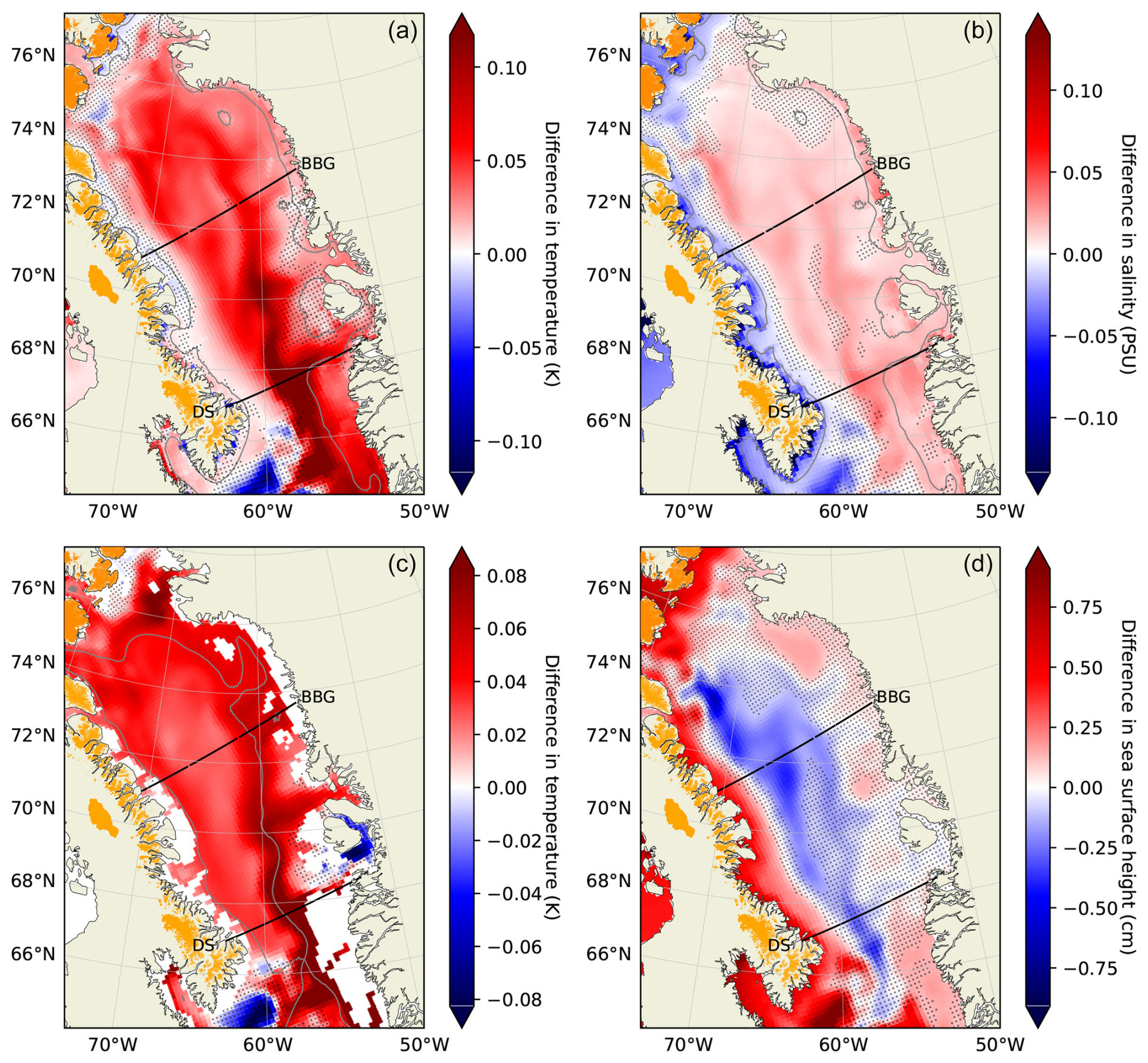
Figure 3 Differences between the halfsolid and noOGGM NEMO runs in Baffin Bay: (a) potential temperature (0–200 m), (b) salinity (0–200 m), (c) potential temperature (200–600 m), and (d) SSH. Dots indicate differences that are not statistically significant, according to Wilcoxon signed-rank tests (p>0.05). BBG stands for the Baffin Bay gyre section and DS for the Davis Strait section. Colored land area indicates glacierized area as recorded in the RGI. Gray lines show the low-pass-filtered 200 m (a, b) and 600 m (c) bathymetry contours. Note the different scales (±3σ) in panels (a) and (c).

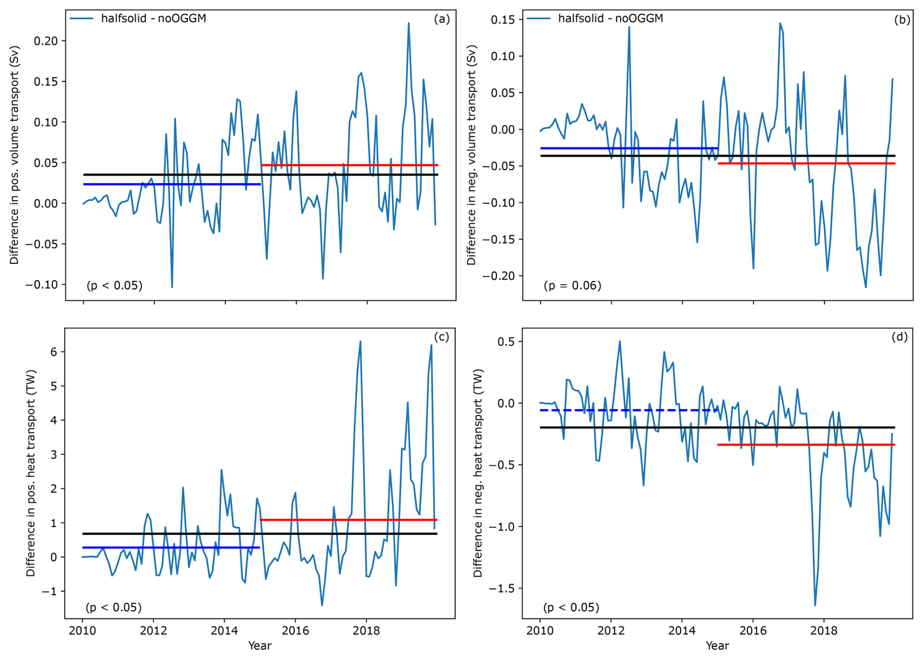
Figure 4 Differences in northward and southward volume and heat transport through Davis Strait between the halfsolid and noOGGM NEMO runs. (a) Northward (positive) volume transport through the Davis Strait (DS) section in Fig. 3, (b) southward (negative) volume transport through DS, (c) northward heat transport through DS, and (d) southward heat transport through DS. The lines show average differences over the first (blue) and last (red) 5 years as well as over all years (black) of the model integrations. Differences between the two NEMO runs that are statistically significant, according to Wilcoxon signed-rank tests (p<0.05), are drawn as solid lines and dashed otherwise. Values in the lower left corners show the p values of Wilcoxon signed-rank tests of differences between the first and last 5 modeled years.

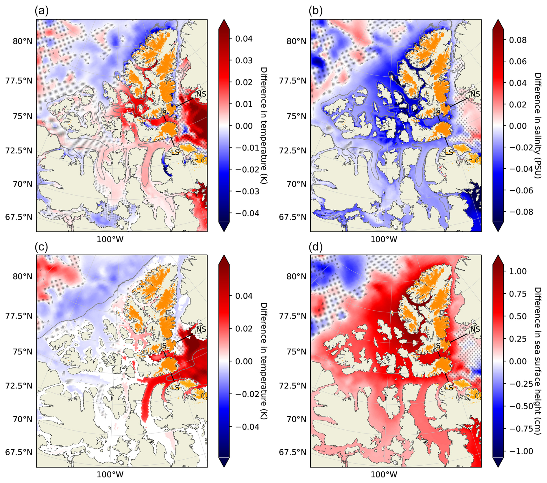
Figure 5 Differences between the halfsolid and noOGGM NEMO runs in the CAA region: (a) potential temperature (0–200 m), (b) salinity (0–200 m), (c) potential temperature (200–600 m), and (d) SSH. Dots indicate differences that are not statistically significant, according to Wilcoxon signed-rank tests (p>0.05). NS stands for the Nares Strait, JS for the Jones Sound, and LS for the Lancaster Sound section. Colored land area indicates glacierized area as recorded in the RGI. Gray lines show the low-pass-filtered 200 m (a, b) and 600 m (c) bathymetry contours. Note the different scales (±3σ) in panels (a) and (c).

3.1.2 Subpolar gyre and AMOC

Figure 6 shows differences in mixed layer depth as well as in density, salinity, and temperature between our two NEMO runs over the upper 200 m in the area of the SPG. The differences in mixed layer depth in the Labrador Sea region between our two NEMO runs, while in part statistically significant, are within the observed interannual variability (Kieke and Yashayaev, 2015). The differences in mixed layer depth are related to the differences in density, which show a varied pattern across the SPG. While in the northern part of the Labrador Sea density is increased, it is decreased in the central and southern Labrador Sea. This is caused by two competing mechanisms: (i) increased import of (cold) fresh water due to the increased input upstream of the Labrador Current caused by glacial melt and (ii) increased entrainment of warm and saline water from the enhanced WGC. There is also more cold and freshwater accumulation in the eastern half of the SPG, resulting in a higher density there. These differences in density are, in turn, translated to differences in the SSH, which show an increase in the central and southern Labrador Sea and a decrease in the northern Labrador Sea and the eastern SPG (see Fig. 7b). Finally, the SSH changes induce changes in the geostrophic circulation, illustrated by the differences in the barotropic streamfunction (BSF; see Fig. 7a). The BSF is increased in the central Labrador Sea, indicating an anticyclonic tendency, while it is slightly decreased in the eastern SPG, suggesting that the center of the gyre circulation shifts slightly in the halfsolid compared to the noOGGM simulation. Though differences in the southeastern parts of Fig. 7 are statistically significant, they show a rather chaotic pattern, reflecting the high eddy activity in this area (Carret et al., 2021).

Further, negative salinity differences in the western Labrador Sea in the 200–600 m depth range (see Fig. A7c) suggest an enhanced recirculation of Labrador Current water (Lavender et al., 2000). In this depth range the warming in the central Labrador Sea due to enhanced import of Atlantic water is more pronounced as well (see Fig. A7d). This partly offsets the freshening from the hypothesized recirculation in that depth range, leading to a weaker density decrease in the central Labrador Sea than in the 0–200 m range, while the enhanced recirculation attenuates the warming due to entrainment of WGC water into the northern Labrador Sea.

Concerning the AMOC, we find no statistically significant difference in northward and southward or total volume flux across 47° N latitude in the Atlantic or the AR7W section across the Labrador Sea (Yashayaev, 2007) and no significant change in the meridional overturning streamfunction. This suggests that there are no significant differences in AMOC strength between the halfsolid and noOGGM experiment. Although we find significant changes in the Labrador Sea's and the SPG's properties, this does not affect the AMOC in a meaningful way. While there were contrasting findings concerning the Labrador Sea's role in affecting the AMOC in previous studies, the differences between freshwater forcings and/or the lengths of our model runs might just not be large enough to have an effect on that large-scale circulation feature (Böning et al., 2016; Garcia-Quintana et al., 2019).

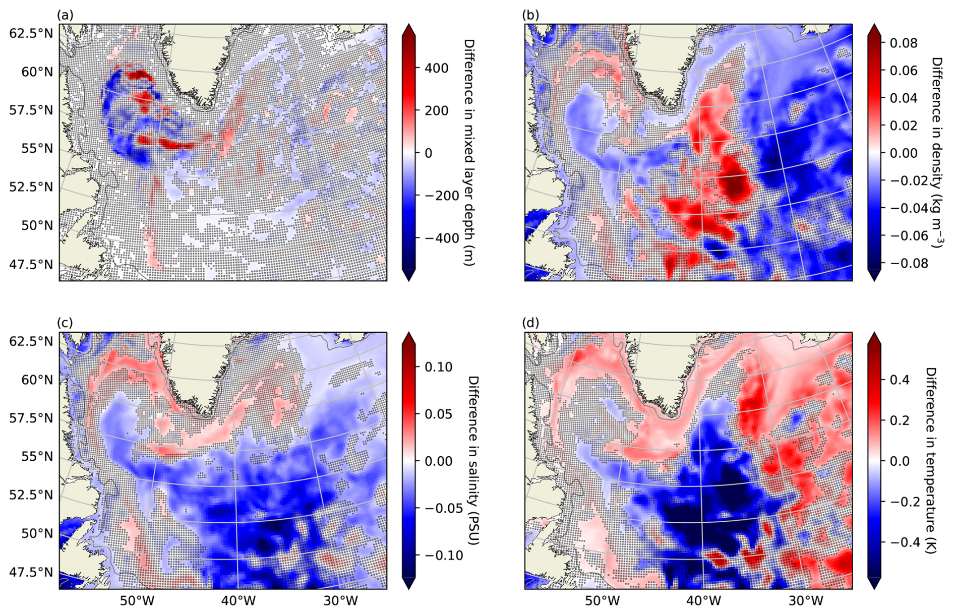
Figure 6 Difference in (a) January–February–March mixed layer depth, (b) density, (c) salinity, and (d) potential temperature averaged over up to 200 m water depth between the halfsolid and noOGGM NEMO runs in the subpolar gyre region. Dots indicate differences that are not statistically significant, according to Wilcoxon signed-rank tests (p>0.05). Gray lines show the low-pass-filtered 200 m bathymetry contours.

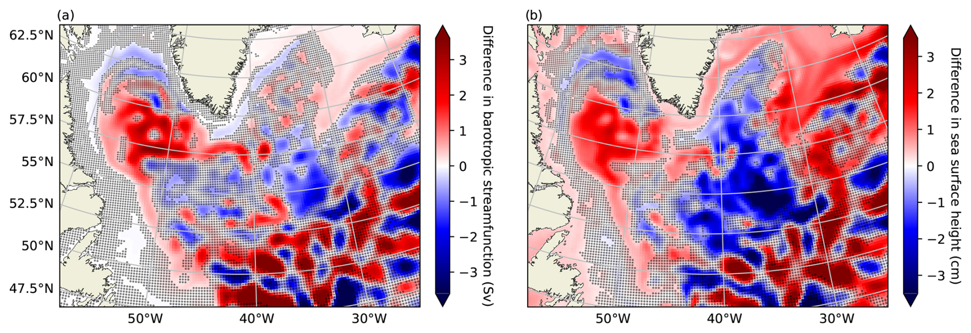
Figure 7 Difference in (a) barotropic streamfunction and (b) sea surface height between the halfsolid and noOGGM NEMO runs in the subpolar gyre region. Dots indicate differences that are not statistically significant, according to Wilcoxon signed-rank tests (p>0.05).

3.1.3 Barents Sea and Nordic Seas

We show the SSH difference between the halfsolid and noOGGM runs in Fig. 8d. The increased freshwater input from Svalbard and the Russian Arctic in the halfsolid run (see Fig. 2) increases the SSH in the northern Barents Sea. This leads to an increased anticyclonic circulation around that area (see Fig. A8), leading, in turn, to a lower volume flux through the Barents Sea Opening (BSO). This is consistent with findings by Lien et al. (2013) and implies a lower (positive) flux of Atlantic water into the Barents Sea, decreasing temperatures in most parts (see Figs. 8a, c and 9a). The volume flux out of the Barents Sea increases (Fig. 9c), leading to a net volume flux decrease of 0.11 Sv (≈4 %). However, some of the additional freshwater input from Svalbard and the Russian Arctic remains in the western Barents Sea and in the Kara Sea (see Fig. 8b).

The Atlantic water not entering the Barents Sea, due to changes in the SSH described above, is routed towards the Fram Strait instead. This leads to an increased northward (positive) volume flux (see Fig. 9b) through Fram Strait. Some of this warm water subsequently enters the Barents and Kara seas from the north (see Fig. 8a), contributing to the increased outflow through the BSO described above. The remainder of the Atlantic water rerouted through Fram Strait roughly follows the eastern Arctic shelf break (see next section). The increase in positive volume flux through Fram Strait begins after roughly half of the NEMO integration time (i.e., 5 years), presumably due to the buildup of meltwater during that period, leading to the increased BSF around Svalbard. This increase in volume flux into the Arctic Ocean through Fram Strait is accompanied by an increased outflux, yielding a net increase in northward (positive) volume flux through Fram Strait of ∼0.24 Sv (≈9 %). The increase in the southward (negative) flux of fresh water through Fram Strait is small and statistically not significant, indicating that the enhanced southward flux is due to enhanced recirculation of Atlantic water. Since not all of the increased volume flux into the Arctic through Fram Strait can be explained by the net positive (eastward) volume flux difference we find for the Barents Sea, we also analyzed the volume fluxes through the Denmark Strait, finding a decrease in southward (negative) and an increase in northward (positive) transport, mainly in the 200–600 m depth range. The net increase of ∼0.10 Sv (≈3 %) through Denmark Strait almost closes the gap between the net decrease in Atlantic water volume flux into the Barents Sea and the net increase in the same into the Arctic Ocean through Fram Strait.

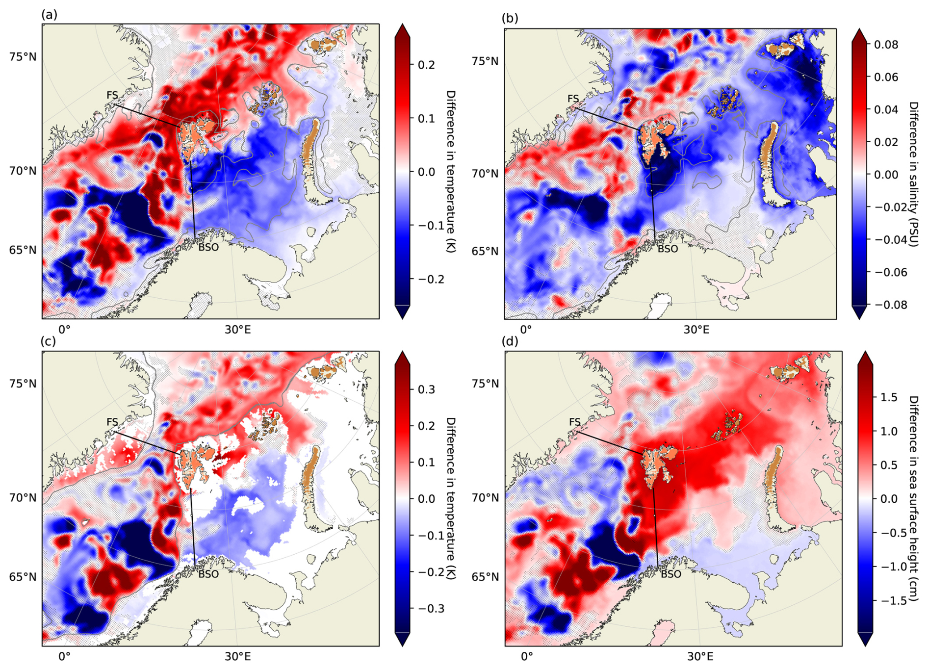
Figure 8 Differences between the halfsolid and noOGGM NEMO runs in the Barents Sea and Nordic Seas area: (a) potential temperature (0–200 m), (b) salinity (0–200 m), (c) potential temperature (200–600 m), and (d) SSH. Dots indicate differences that are not statistically significant, according to Wilcoxon signed-rank tests (p>0.05). FS stands for Fram Strait and BSO for the Barents Sea Opening. Colored land area indicates glacierized area as recorded in the RGI. Gray lines show the low-pass-filtered 200 m (a, b) and 600 m (c) bathymetry contours. Note the different scales (±3σ) in panels (a) and (c).

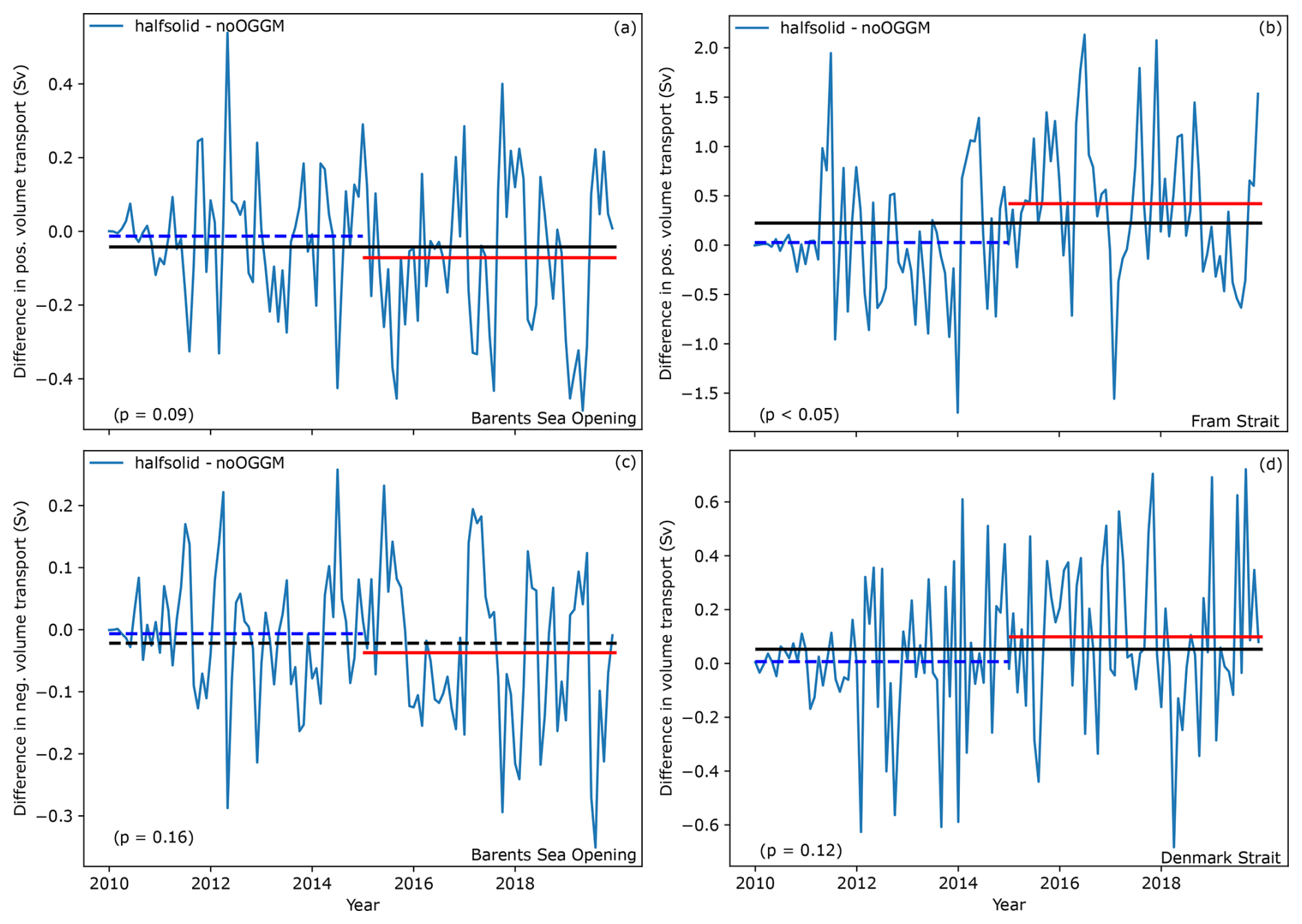
Figure 9 Difference in positive transport through (a) the Barents Sea Opening (BSO) and (b) Fram Strait (FS) in (c) negative volume transport through the BSO and (d) total volume transport through Denmark Strait between the halfsolid and noOGGM NEMO runs. Positive transport through FS and Denmark Strait means northward, while positive transport through BSO means eastward. The horizontal lines show average differences over the first (blue) and last (red) 5 years, as well as over all years (black) of the model integrations. Differences between the two NEMO runs that are statistically significant, according to Wilcoxon signed-rank tests (p<0.05), are drawn as solid lines and dashed otherwise. Values in the lower left corners show the p values of Wilcoxon signed-rank tests of differences between the first and last 5 modeled years.

3.1.4 Arctic Ocean, sea ice, and icebergs

We find a band of warmer water in the halfsolid run in the eastern part of the Arctic Ocean that follows the shelf break (Arctic Circumpolar Current; see Fig. 10a, c) and is caused by the increased import of Atlantic water through Fram Strait, which is discussed in the previous section. The warm Atlantic water also reaches further north up to the Lomonosov Ridge in the 200–600 m depth range (see Fig. 10c). Inspecting differences in salinity, a patch of increased salinity north of the New Siberian Islands and around the Mendeleev Ridge is visible (see Fig. 10b). This causes a decreased SSH in that area (see Fig. 10d) through an increase in density. The changes in salinity and in SSH displayed in Fig. 10b and d can be explained by the enhanced Arctic Circumpolar Current, as it blocks the export of fresher water from the Laptev shelf to the interior of the Arctic Ocean. This leads to the saltier water from the Atlantic being accumulated on the East Siberian Shelf and around the Mendeleev Ridge, while more fresh water stays on the eastern Arctic shelves, where we see decreased salinity and increased SSH.

The largest decreases in sea ice thickness between the two NEMO simulations can be found in the western Greenland Sea, north of Svalbard, and in the CAA (Fig. 11). The decrease in sea ice thickness in the former two areas is caused by the changes in the pathway of Atlantic water in the Nordic Seas. Enhanced transport through Fram Strait and enhanced recirculation towards Greenland's east coast increase the advection of heat in these regions (see Fig. 8a, c). However, we also find a decrease of 1 % in the southward (negative) sea ice velocity's absolute value across Fram Strait (p<0.05; not shown), indicating an influence of the changes in ocean dynamics. Wang et al. (2020) identified a positive feedback, linking an increased import of Atlantic water through Fram Strait to a sea ice decline in that area, which might also play a role here. In the CAA region, we find a similarly strong decrease in sea ice thickness. The smaller increase in upper-layer temperature in the CAA compared to the Fram Strait and eastern Greenland areas suggests that factors other than increased ocean heat content play a role there. The decrease in ice thickness in the CAA is driven by less sea ice advection, since the increase in SSH across the region leads to a divergent flow out of the area (see Figs. 5d and A9). This is also reflected in Fig. A10, showing more sea ice production in the CAA area in the halfsolid run. As expected from the higher temperatures in Baffin Bay in the halfsolid run, the sea ice is slightly thinner in this area as well, although differences in sea ice production are heterogeneous (see Fig. A10). This indicates that dynamical factors, i.e., more southward sea ice transport through Davis Strait, also play a role here. The only area where we find a slightly increased sea ice thickness is between the Barents and Kara seas, which is most probably related to the decreased heat transport into Barents Sea due to the rerouting of Atlantic water described above. Sea ice production (growth) can be influenced by several processes (e.g., Cornish et al., 2022): upper-ocean stratification regulating the amount of thermal forcing supplied to the ice–ocean interface, the negative ice thickness–growth feedback, the relationship between ice thickness–growth and ice drift, and ocean water's freezing point being a function of its salinity. The increased vertical mixing we apply in our model setup at locations where fresh water enters the ocean and differences in latent heat extracted from the ocean due to differences in iceberg melt can also affect sea ice production locally. This list of processes is non-exhaustive, and pinning the differences in sea ice thickness and production to individual processes is out of the scope of this work. The net difference in sea ice thickness in the Northern Hemisphere between the two NEMO experiments is still intriguing, since we only add fresh water to the ocean, which should not increase its heat content. This suggests that increased high-latitude freshwater input due to glacial melt (outside the ice sheets) can decrease sea ice thickness through the changes in ocean circulation it induces.

Figure A11 shows areas of statistically significantly increased iceberg melt around Svalbard and the Russian Arctic islands, as expected from the difference in calving input between the halfsolid and noOGGM simulations. Moreover, we find more iceberg melt throughout the Arctic Ocean, although this is not statistically significant. Since the presence of icebergs from Greenland in Baffin Bay and the CAA straits is already large, the addition of calving from the CAA in the halfsolid NEMO does not significantly alter the iceberg melt pattern in that region.

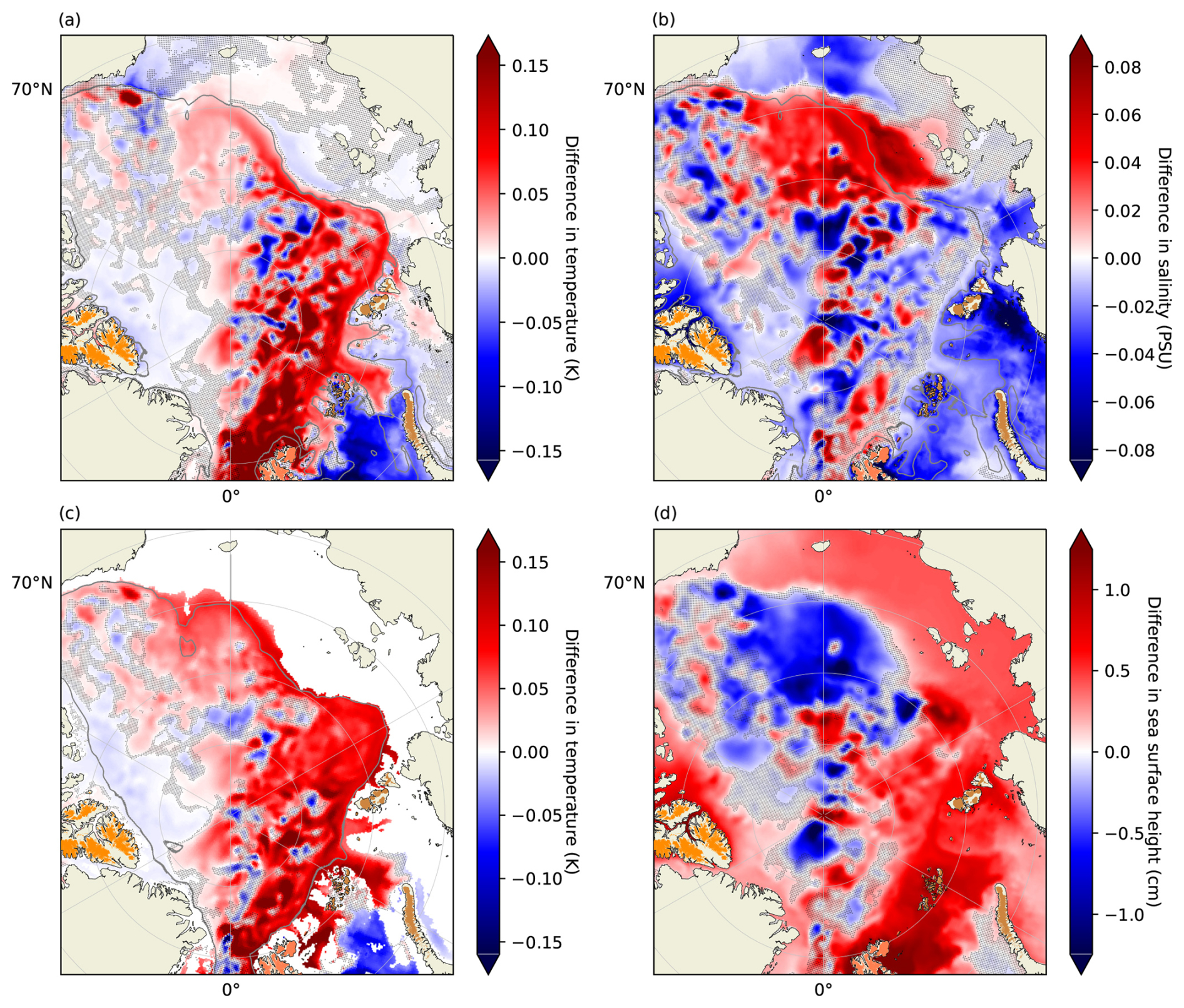
Figure 10 Differences between the halfsolid and noOGGM NEMO runs in the Arctic Ocean area: (a) potential temperature (0–200 m), (b) salinity (0–200 m), (c) potential temperature (200–600 m), and (d) SSH. Dots indicate differences that are not statistically significant, according to Wilcoxon signed-rank tests (p>0.05). Colored land area indicates glacierized area as recorded in the RGI. Gray lines show the low-pass-filtered 200 m (a, b) and 600 m (c) bathymetry contours. Note the different scales (±3σ) in panels (a) and (c).

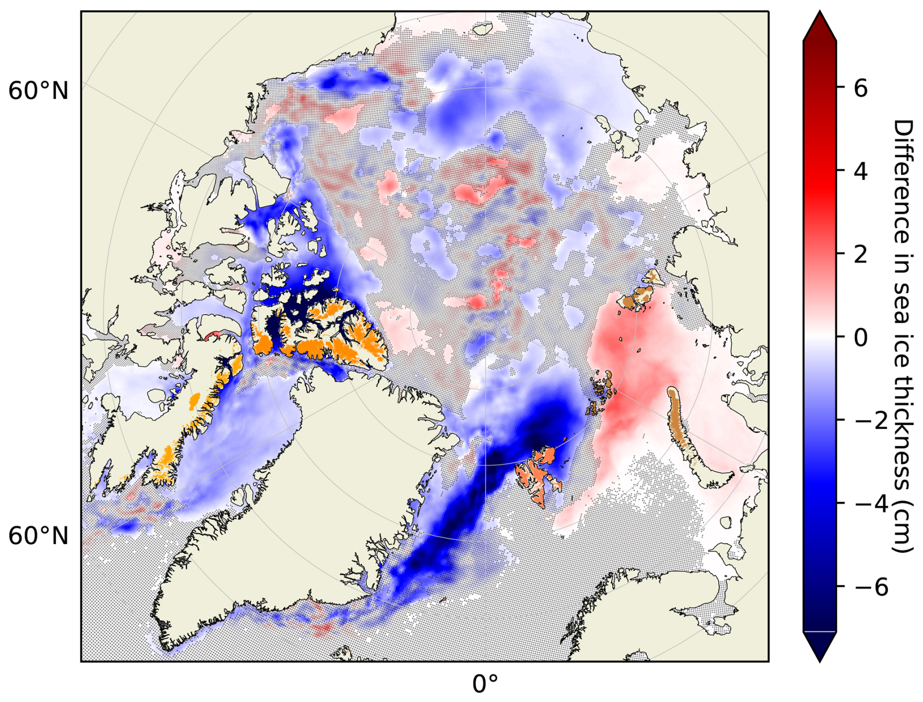
Figure 11 Difference in sea ice thickness between the halfsolid and noOGGM NEMO runs. Dots indicate differences that are not statistically significant, according to Wilcoxon signed-rank tests (p>0.05). Colored land area indicates glacierized area as recorded in the RGI.

3.2 Glacier model

Figure 12 and Table 1 show the results of our OGGM runs with the submarine melt parameterization described above. Submarine melt accounts for between 10 % and 27 % of total frontal ablation according to the method we applied, exhibiting a relatively large interquartile range of the results with different valid parameter sets from the Latin hypercube sampling. We find the lowest median submarine melt fraction in Arctic Canada North (12 [10, 30] %; the value in square brackets is the interquartile range) and the highest in Arctic Canada South (35 [18, 44] %). Note that we exclude Flade Isblink from our results for the Greenland periphery here, as its RGI outlines are erroneous and it maintains an ice shelf (Möller et al., 2022), making the dynamical modeling of it problematic in our framework. Tables 1 and 2 provide an indication of the prevalent frontal ablation mechanisms in the different regions (i.e., submarine melt vs. iceberg calving). That we estimate the largest fraction of frontal ablation caused by submarine melt for the region Arctic Canada South, but the highest thermal forcing for Svalbard, indicates that in the latter region frontal mass loss is more dynamically driven. That is because in OGGM, volume below flotation at the front is removed and added to the calving output variable (i.e., no ice shelves can form). Therefore, if much ice is removed by the flotation criterion, less can be removed by submarine melt when total frontal ablation rates are constrained with observational estimates. The amount of ice above the water level at the front also plays a role here though, since only ice below the water level can be removed by submarine melt.

Table 1 shows that there is no large difference in the submarine melt estimates when applying the thermal forcing derived from the noOGGM runs compared to the runs forced with the halfsolid NEMO output. This suggests that there are only small coupling effects on glacier mass change over the decadal timescale we investigated here. Table 2 shows that the differences in thermal forcing in the vicinity of marine-terminating glaciers are small on average over the last 5 years of the NEMO integration. We find the largest increase in Svalbard, caused by the rerouting of warm and saline Atlantic water from the southern Barents Sea Opening to the Fram Strait, where some of it enters the Barents Sea from the north close to Svalbard (see Fig. 8a, c). This is also the region where we find the strongest increase in submarine melt using the halfsolid NEMO run output compared to the noOGGM output (see Table 1). In contrast, thermal forcing is slightly decreased in the halfsolid run in Arctic Canada North and the Russian Arctic. In the latter case this is due to less heat transport from the Atlantic into the Barents Sea. Tables 1 and 2 furthermore indicate a perceptible influence of the dependence on water depth in Eq. (2). For example, in Arctic Canada South we find less of an increase in submarine melt in the third than in the first quartile comparing the halfsolid to the noOGGM NEMO run. This is probably because with stronger submarine melt, we simulate stronger retreat of marine-terminating glacier fronts due to undercutting, which, depending on the submerged bed topography, can decrease the water depth. This leads to a decreased sensitivity to subglacial discharge in Eq. (2), while the amount of subglacial discharge is the same in both OGGM simulations. The Greenland periphery is the only region for which we find a smaller absolute percentage change in submarine melt rates than in thermal forcing (see Tables 1 and 2), likely indicating that in this region subglacial discharge has a stronger influence on submarine melt in our model than in the other regions.

Table 3 displays the median and interquartile range of valid parameter sets we find in the different regions as well as the median and interquartile range of the number of valid parameter sets found per glacier. It shows that there are differences between the regions for the parameters B, β, and to a minor extent A, which are related to the efficiency of heat transfer from the open ocean into the glacier front and the increase of this heat transfer due to subglacial meltwater discharge. The Greenland periphery and Arctic Canada South exhibit the largest median (and third quartile) values for A and B. Moreover, we generally find more valid parameter sets for the glaciers in the Greenland periphery and Arctic Canada South. Those findings point to regional differences in the valid parameter ranges, and it appears to be the case that the parameter range could be adjusted for the individual regions and glaciers. While our aim in this work was to produce a first estimate of submarine melt of glaciers outside the GrIS, finding more accurate parameter values for the parameterization warrants further investigations in the future.

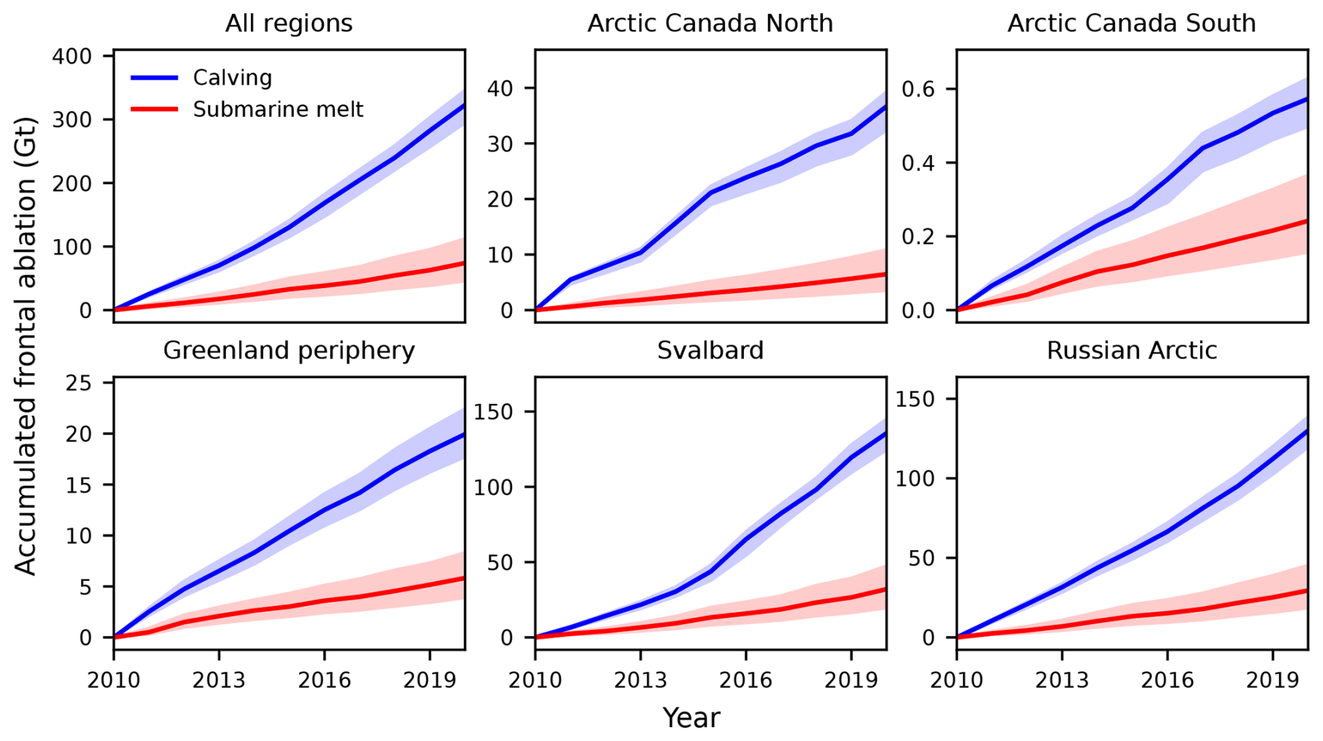
Figure 12 Estimated amounts of the two frontal ablation components submarine melt and calving. Solid lines represent the median and shading the interquartile range of the valid parameter sets. Note the different scales for the different regions.

Table 1 Estimates of submarine melt rates (median, with the interquartile range in brackets) between 2015 and 2019 of marine-terminating glaciers in the NEMO-ANHA4 domain. Q_sm represents submarine melt rates, Q_fa the total frontal ablation rates, and ΔQ_sm the difference in submarine melt rates between the halfsolid and noOGGM NEMO runs over the period. n is the number of marine-terminating glaciers in the region.

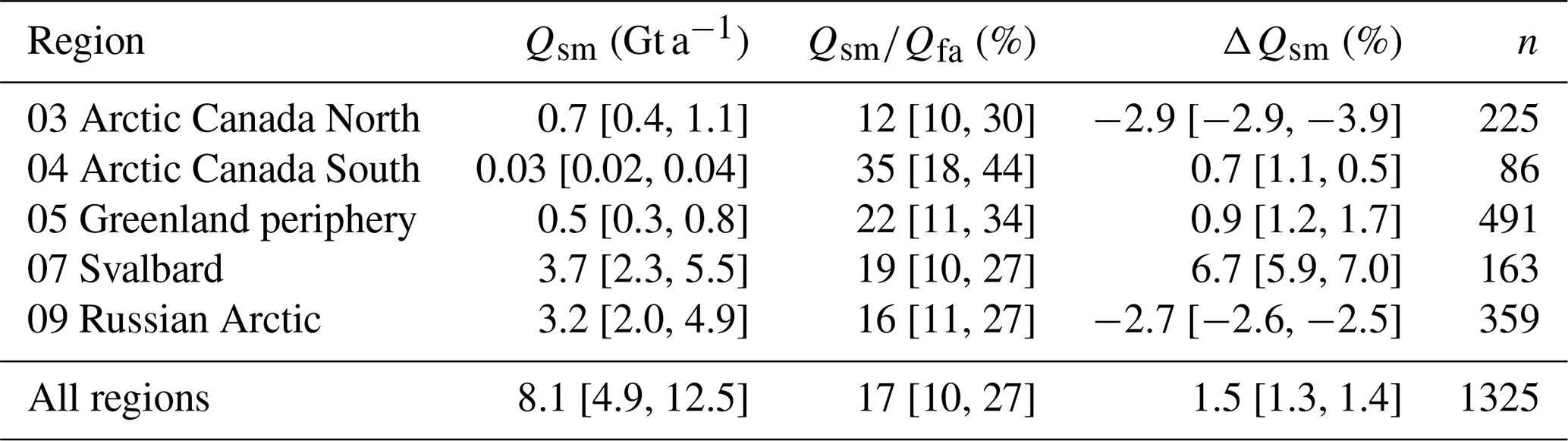
Table 2 Average of ocean variables in the vicinity of marine-terminating glacier fronts over 2015 to 2019, weighted by submerged frontal cross-sectional area. T_f is thermal forcing, T potential temperature, S salinity, and d_o the distance-averaged ocean depth of grid cells taken into account for the calculation. The percent difference between the halfsolid and noOGGM NEMO runs (i.e., halfsolid minus noOGGM) is given in parentheses.

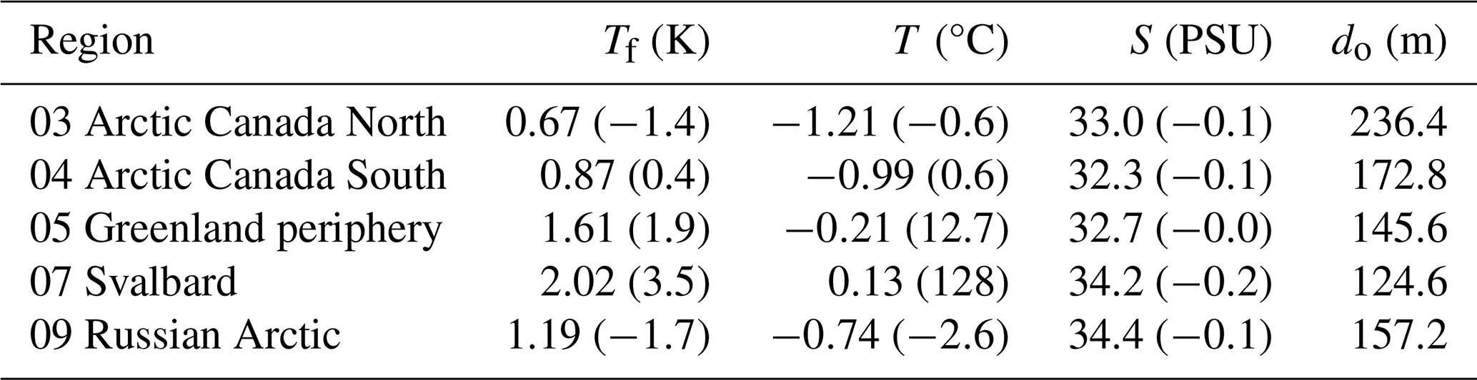
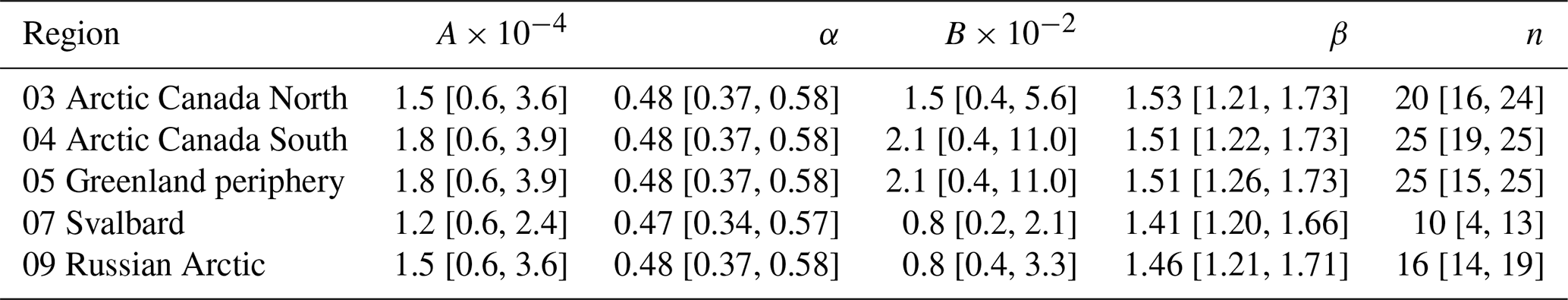
Table 3 Ranges (median, with the interquartile range in brackets) of parameter values in Eq. (2) complying with total frontal ablation estimates from satellite-derived observations (Kochtitzky et al., 2022). n is the median number of valid parameter sets found for individual glaciers in the regions.

4 Discussion

4.1 Ocean model results

4.1.1 Baffin Bay and Canadian Arctic Archipelago

Concerning Baffin Bay, we compare our results to those of Castro de la Guardia et al. (2015), who investigated the impact of increased freshwater input along the (west) coast of Greenland on the Baffin Bay circulation and its exchanges with the Arctic through the CAA. They found an increase in heat transport into Baffin Bay through Davis Strait and a reduction in volume fluxes through the CAA into Baffin Bay, both related to an increase in the Baffin Bay gyre's strength. We find a smaller increase in Baffin Bay temperatures (∼0.1 vs. ∼0.3 K), which can be explained by the smaller increases in sea surface height gradients and stratification, since our additional freshwater input to Baffin Bay is roughly a factor of 5 (50) smaller compared to their experiment with the lowest (highest) additional freshwater forcing along Greenland's west coast. Interestingly, the increase in northward heat transport through Davis Strait we find is higher (1.1 vs. 0.5 TW), but the average warming in Baffin Bay is smaller than the differences diagnosed by Castro de la Guardia et al. (2015). This points to the significance of changes associated with an increasing SSH gradient and stratification of Baffin Bay in moderating the temperature response to increased heat influx. The decrease in volume flux through the CAA into Baffin Bay (∼0.8 %) is also small compared to the 9 % to 46 % in the experiments demonstrated by Castro de la Guardia et al. (2015). Volume flux through the CAA into Baffin Bay was found to be mainly controlled by the SSH gradients across the straits connecting Baffin Bay to the Arctic Ocean (McGeehan and Maslowski, 2012; Hu and Myers, 2014), suggesting that these gradients did not change sufficiently to alter the total volume flux between the Arctic and Baffin Bay in a notable manner when comparing our two NEMO experiments.

4.1.2 Nordic Seas and Arctic Ocean

Our findings are also consistent with those of Lien et al. (2013), linking the effect of changes in SSH around Svalbard to changes in the partitioning of the Atlantic water inflow to the Arctic through the BSO and Fram Strait. Regarding the sea ice thickness differences between our halfsolid and noOGGM NEMO experiments, it is intriguing that Labe et al. (2018) find negative trends of sea ice thickness between 1979 and 2015 in some similar areas. These areas are (north)western Queen Elizabeth Island in the CAA and north of Svalbard. This might hint at the fact that increased freshwater input from glaciers outside Greenland is a relevant process for (regional) sea ice thickness changes. Concerning the patch of increased salinity in the Arctic Ocean's upper 200 m (see Fig. 10b), similar changes in (near-)surface salinity have been found in previous studies on the impact of increased freshwater input from Greenland (Devilliers et al., 2024; Swingedouw et al., 2013).

4.1.3 Subpolar gyre

While there have been numerous studies on the effect of Greenland melt on modeled Labrador Sea convection and subsequently the AMOC, it is not straightforward to compare their results to ours. That is because in this study we focus on the impact of fresh water added in different locations, which naturally leads to different impacts on the ocean circulation. Still, one location that is comparable is the SPG and Labrador Sea region, as at least some fraction of the additional fresh water we included in the halfsolid run will impact that area. We see that the patterns in SSH differences between our two runs are qualitatively consistent with previous studies (Saenko et al., 2017; Stammer et al., 2011). This pattern consists of a larger SSH in the Labrador Sea and western SPG area and a lower SSH in the eastern SPG (see Fig. 7). The differences in mixed layer depth we find are also consistent with previous studies (Schiller-Weiss et al., 2024; Devilliers et al., 2021). The mixed layer depth is decreased in the Labrador Sea and increased in the eastern SPG, though this increase is not statistically significant in our case (see Fig. 6). Areas of increased mixed layer depth that are intertwined with the areas of negative differences in the Labrador Sea are also presented in Schiller-Weiss et al. (2024), while they are not in Devilliers et al. (2021). Using a freshwater forcing around Greenland similar to the one used in Devilliers et al. (2021), but a different climate model, Devilliers et al. (2024) find the opposite mixed layer depth response (increase in the Labrador Sea and decrease in the eastern SPG). Overall, these comparisons with previous studies suggest that the additional fresh water from glacial melt outside Greenland in the halfsolid run might exacerbate the impact of increasing Greenland freshwater input in the Labrador Sea and SPG area.

Placing our results for the SPG circulation (see Figs. 6 and A7) further in the context of the existing literature, we find that the decrease in SSH and the increase in density of the upper 600 m in the eastern SPG resemble patterns that were linked to an increase in its overall strength (Hakkinen and Rhines, 2004; Chafik et al., 2022; Foukal and Lozier, 2017). The changes in SSH and density could be related to the stronger WGC we find in the halfsolid compared to the noOGGM run, although an increase in the SPG's overall strength is not directly apparent from the differences in the BSF we find. Moreover, the pattern of increased salinity around the northern SPG resembles the pattern found by Born et al. (2016) comparing a strong to a weak mode of the gyre. Thus, we speculate that a relation between the density patterns in the SPG and its circulation features is reflected in our results. The proposed relation is as follows: due to decreased density, in our case caused by increased freshwater input, SSH increases in the Labrador Sea. Now, Chafik et al. (2022) demonstrated that water leaves the Labrador Sea eastwards through two main pathways: either via the rim current that follows the boundary of the SPG or through the gyre's interior. Hence, the decreased density in the Labrador Sea leads to more of the water that is cooled by surface heat loss, but does not sink, in the Labrador Sea being accumulated in the eastern SPG together with fresh and cold water from upstream of the Labrador Current. In turn, increased density and decreased SSH in the eastern SPG causes more Atlantic water to move around the gyre's eastern part and towards the Labrador Sea. Sun et al. (2021) proposed oscillating feedbacks of the SPG's strength and the deep convection in the Labrador Sea, asserting that an increased gyre strength leads to an increased density transport into the Labrador Sea, in turn increasing the deep convection. This would decrease SSH in the Labrador Sea and the export of cooled water to the gyre's interior. In our results, some areas of the northeastern Labrador Sea indeed show a slightly higher density and mixed layer depth, hinting at this feedback potentially being in effect. While, as stated above, the changes in mixed layer depth and the BSF are not straightforward, the coherence of our findings with mechanisms linking Labrador Sea deep convection and the SPG's strength presented in previous publications is intriguing. Further research might be conducted to investigate whether the positive feedback of the oscillation mechanism proposed by Sun et al. (2021) can offset increased freshwater input over a longer time span.

4.2 Ocean model setup

We did not aim to produce hindcasts that are as accurate as possible but to obtain first estimates of the coupling effects between OGGM and NEMO, for which we consider a somewhat idealized setup appropriate. Although we deem our rather simple approach sufficient to produce first estimates of the coupling effects between OGGM and NEMO on a decadal timescale, we now lay out some aspects that could be improved in future works on the subject of Northern Hemisphere ice–ocean interactions outside the GrIS.

4.2.1 OGGM to NEMO

Concerning the aspect of using OGGM output as an input for NEMO, it is arguable whether putting the meltwater runoff and calving estimates derived from OGGM simply into the top level of the NEMO grid cell nearest to the glacier terminus is a sound approach. Particularly in regions with complex topography and/or fjord systems, for example the CAA, more sophisticated routing approaches might be advisable. In addition, some of the fresh water might evaporate or seep into the ground upstream. Whether the halfsolid assumption is valid for regions outside Greenland also needs to be investigated, since it is not clear how much of the iceberg mass actually melts within the fjords before the icebergs reach the open-ocean NEMO grid cell. When differentiating between solid and liquid discharge, the amount of submarine melt should be taken into account as well.

We implicitly assume that the amount of submarine melt of glaciers outside the GrIS is so small that the amount of heat drained from the ocean necessary to produce this melt is negligibly small for the ocean heat budget. A rough estimate indicates that approximately 2.9×10¹⁸ J a⁻¹ would be needed for our median estimate of 8.1 Gt a⁻¹ submarine melt. This is 3 orders of magnitude smaller than the estimated annual ocean heat uptake due to anthropogenic climate change (Cheng et al., 2022), indicating that the impact of submarine melt from glaciers outside the ice sheets is small on the global scale of the ocean heat budget, though it might be relevant on a local scale. Similarly, it would be interesting to see what the effect of adjusting the freshwater input's temperature to values different from the ocean surface temperatures is. Glacial meltwater might actually be colder, and thus such an adjustment might have an influence on the model results.

Moreover, it might be the case that the increased surface layer mixing in all NEMO grid cells where we add liquid fresh water to the ocean is inaccurate. That is because in reality, the glacial meltwater is injected into the fjords, which is some distance apart from the open ocean, and the meltwater might be stored in the fjords for some time before being released to the ocean (Straneo and Cenedese, 2015; Sanchez et al., 2023). Thus, increased surface mixing might not actually occur at the open-ocean locations where it is added to the NEMO-ANHA4 grid in our simulations. As surface and submarine melt of marine-terminating glaciers enter the fjords at depth and is subsequently mixed, the modeling setup could be enhanced by a more accurate representation of meltwater injection at depth, especially when individual fjords are not resolved in the ocean model.

4.2.2 Forcing data, resolution, and further analyses

The baseline runoff and the Bamber et al. (2018) data not covering the whole modeling period might induce some uncertainty in our results, since the impact of the additional fresh water we examined could be altered. If, for instance, the ratio of the additional fresh water in the halfsolid run to the baseline plus Greenland runoff was larger (smaller), the impact would presumably be larger (smaller) as well.

Another aspect that could be improved regarding the modeling approach is the resolution of the ocean model because the NEMO-ANHA4 setup is probably too coarse to yield a good representation of ocean eddies, which is of importance for processes in, for instance, the Labrador Sea (Pennelly and Myers, 2022), the Fram Strait (Hattermann et al., 2016), and the Arctic Circumpolar Current (Athanase et al., 2021). Concerning transports across the CAA, Hu et al. (2019) showed that twin $\mathrm{1}/\mathrm{4}$ and $\mathrm{1}/\mathrm{12}$° simulations were similar in this regard. Furthermore, employing a fully coupled ocean–atmosphere model could provide insights into how ocean–atmosphere interactions might modulate the findings described in this work. Applying (passive) tracers in future studies could additionally reveal where the meltwater from the glaciers moves in the ocean.

As alluded to in Sect. 3.1.2, statistically significant changes can arise from chaotic variability. For instance, in regions with high eddy activity, areas of statistically significant differences might reflect a chaotic shift of individual eddies rather than a systematic response to the freshwater forcing. Running a suit of different model setups would increase the confidence in the (statistical) significance of this work's findings. One approach could be to run the same model setup several times, but applying different atmospheric forcing datasets, e.g., as in Pennelly and Myers (2021). Finally, a thorough evaluation of the model results with observations could reveal whether the inclusion of glacial melt runoff outside Greenland actually enhances the model's fidelity.

4.2.3 Simulation length

Longer model runs would provide insights into whether the accumulation of fresh water from glacier melt outside of Greenland could at some point influence the AMOC either directly due to density changes at deepwater formation sites or mechanisms linked to the reduction of Arctic sea ice cover (Sévellec et al., 2017) and whether the impacts we find persist on longer timescales. Conducting coupled simulations over a climate period (30 years) would also attenuate compounding effects of internal variability and the imposed forcing. For instance, during our chosen modeling period, there were periods of freshening (2012–2016; Holliday et al., 2020) and cooling or warming (2014–2016, 2016–2018; Desbruyères et al., 2021) in the subpolar North Atlantic due to natural variability on (multi-)decadal timescales. These might modify the ocean's response to the difference in freshwater forcing between our two NEMO experiments. The mechanism described by Holliday et al. (2020), linking the aforementioned freshening to changes in the Labrador Current's pathway due to wind stress forcing, in particular could have an impact on the distribution of the fresh water added to the current upstream. The issue of natural variability might also be related to why we see a change in the sign of the differences in the WGC's strength between our two model setups after the first 5 years (see Fig. A5). Combining the mentioned potential improvements with a longer integration time of NEMO would consolidate knowledge about the influence of glaciers outside the GrIS on the ocean circulation and make sure potential initial adjustment and spin-up effects have fully abated.

4.2.4 Spin-up

The spin-up of the ocean model has two main aspects. Firstly, the model is initialized with ocean reanalysis data and forced by atmospheric reanalysis data. Since even in more recent times observations of the deep ocean are sparse, the initial conditions might be inconsistent with the model physics. Additionally, the initial conditions might be inconsistent with the atmospheric forcing. This means that the modeled ocean state adjusts to these inconsistencies in what can be called an initialization shock, which levels off relatively quickly in our setup though (see Fig. A12). Any remaining drift due to initialization will be similar in our two setups, thus likely not hindering a meaningful comparison between them regarding the impact of increased freshwater input at the surface. The second aspect is the accumulation of this additional fresh water in the ocean. The larger freshwater input in the halfsolid run will have an increasingly strong effect over time, while the ocean (model) adjusts to this forcing. An indication of both our model setups starting to follow their own trajectory after the first half of the modeled period is that differences between them shown in Fig. 9 are not statistically significant in the first 5 years, but they are in the second 5 years. Generally, spin-up refers to a procedure that brings a general circulation model (close) to an equilibrium state, and this is particularly intricate for the deep ocean. In this study, we examined an ocean perturbed by anthropogenic climate change and did not focus on the deep ocean. Moreover, we start the model from contemporaneous conditions, which should be relatively well constrained for the upper ocean. Therefore, we argue that 10 years of a model run, considering the first 5 years as spin-up, is suitable for a first-order estimate of the ice–ocean interactions near the surface that we studied. Still, it should be investigated in future studies whether running the model with constant forcing over several years and then switching to the actual forcing time series would significantly alter the findings.

4.3 Glacier model

On the side of OGGM, it is apparent from Table 3 that the parameter ranges sampled with the Latin hypercube approach should be adjusted for individual regions. Xu et al. (2013) also suggest that the parameter values might actually differ between (high and low) subglacial discharge regimes. Moreover, the parameters in Eq. (2) probably depend on processes like subglacial hydrology and frontal plume formation, fjord circulation and subglacial discharge's effect on it, and fjord–ocean water interchange as well as the fjord geometry. As we find the largest regional differences in the parameters that control the efficiency of heat transfer from the open ocean into the glacier front in the absence of subglacial discharge (B and β), the differences in parameter values might be best explained by differences in fjord properties and fjord–ocean exchange. Since resolving individual fjords in an ocean circulation model would necessitate a very fine spatial resolution, it is too computationally expensive to run such a setup for all the relevant fjords and longer time periods. This points to the fact the fjord water properties in relation to open-ocean water properties and subglacial discharge need to be better understood and incorporated in models in order to better constrain the involved parameters. Another aspect that could be further investigated concerning the submarine melt parameterization is which part of the ocean in the marine-terminating glaciers' vicinity should be used to source the thermal forcing from before inserting it in Eq. (2). Refining the distance from the glacier termini as well as the ocean depth range that should be taken into account could help to better constrain submarine melt estimates.

Furthermore, dynamically modeling marine-terminating glaciers requires additional parameters compared to land-terminating glaciers that need to be constrained and might be interrelated. For instance, the frontal ablation parameter (k) depends on the choice of values for the parameters involved in the modeling of ice dynamics, since these parameters control the initial geometry given by the ice thickness inversion as well as the dynamical mechanisms of frontal ablation (Malles et al., 2023). This means that when aiming at most accurately simulating (frontal) ice dynamics, such parameters need to be better constrained, although this was not the aim in this work.

4.4 Future projections

An obvious next step is the continuation of the simulations into future projections, since glacier mass loss is projected to increase in the future and hence the impact of increased freshwater input can be expected to grow (Marzeion et al., 2020). For this, a coupling scheme that updates the forcings between the models, for example in the form of a decadal step coupling, would have to be developed. Regarding projections of future glacier mass loss, it would be interesting to investigate how future changes of ocean properties (different from the effects caused by the meltwater) will influence projected frontal ablation rates. For example, increased thermal forcing in combination with increased subglacial discharge would increase submarine melt rates, which might lead to stronger undercutting and thus accelerated retreat (Wood et al., 2021, 2018). On the other hand, the number of marine-terminating glaciers outside the GrIS is already decreasing and projected to continue decreasing in the future (Kochtitzky et al., 2022; Malles et al., 2023), which might attenuate the potential increase in submarine melt.

5 Conclusions

We have presented the first investigation of ice–ocean interactions in the Northern Hemisphere outside the GrIS by applying one-way coupling of an ocean general circulation model (NEMO-ANHA4) and a glacier evolution model (OGGM) for the years 2010 to 2019. On the ocean side, we find that the NEMO simulation forced with freshwater input derived from glacier mass loss estimates given by OGGM shows considerable differences from the experiment solely forced with freshwater input from the GrIS. Consistent with what has been found in a previous study on the influence of increased freshwater input from the western GrIS on Baffin Bay (Castro de la Guardia et al., 2015), we find an increased ocean heat content in this region. We also find changes in the Nordic Seas that are brought about by the increased freshwater input around Svalbard and the Russian Arctic that lead to a decreased transport of Atlantic water into the Barents Sea, causing this water to be rerouted through Fram Strait into the Arctic. Furthermore, we find sea surface height changes in the Baffin Bay, the CAA, the Nordic Seas, the subpolar gyre, and the Arctic Ocean that indicate changes in (gyre) circulation patterns across the Northern Hemisphere. Concerning the AMOC, our results do not suggest a significant change and the decrease in mixed layer depth over the Labrador Sea region in the OGGM-forced NEMO simulation falls within the range of natural variability. Regarding the Arctic Ocean, an intrusion of rerouted warm Atlantic water through Fram Strait leads to a band of warmer water along the eastern shelf break. This rerouting of Atlantic water also results in a decrease in sea ice thickness in the Fram Strait region and north of Svalbard. We also find a comparatively strong decrease in sea ice thickness in the CAA. In total, sea ice thickness is decreased in the Northern Hemisphere when including freshwater forcing from glacial melt outside the GrIS.

Regarding the influence of the oceanic forcing on glacier mass loss, we find that for marine-terminating glaciers in the domain of the NEMO-ANHA4 configuration, submarine melt accounts for a median 17 % (≈8.1 Gt a⁻¹) of frontal ablation throughout the spun-up simulation period (2015 to 2019), with an interquartile range of 10 % to 27 % (≈4.9 to 12.5 Gt a⁻¹). The increase in submarine melt when applying the thermal forcing from the NEMO experiment that includes freshwater input from the OGGM glaciers, compared to the experiment that does not include it, is small (1.5 [1.3, 1.4] %). The only region where we find a notable increase in submarine melt is Svalbard. This is caused by the rerouting of warm Atlantic water through Fram Strait, which thereby reaches Svalbard from the north. On the other hand, we find a slight decrease in Arctic Canada North and the Russian Arctic. Our results suggest that the ranges applied in the Latin hypercube sampling of the newly implemented parameterization's estimated parameter space should be adjusted for the individual regions. We find less viable parameter sets for individual glaciers in some regions than in others when applying the same ranges for all regions.

Future studies investigating Northern Hemisphere ice–ocean interactions could improve several aspects of this work. Using a (more rigorously spun-up) higher-resolution ocean model configuration and analyzing passive tracer movements could yield stronger insights into the impact of increased freshwater input from glacier mass loss outside the GrIS on ocean circulation. Additionally, advancing the simulations into future projections would be crucial in gaining a better understanding of potential future changes in the ocean as well as in glacier mass changes due to ice–ocean interactions. This would necessitate an actual two-way coupling of the models, for example through decadal step coupling. Another approach could be to conduct decadal snapshot simulations similar to what was presented in this work, but for a future period in which the melt signal from Northern Hemisphere glaciers outside Greenland will be larger. Such a snapshot approach would avoid the computational cost of long transient simulations but might not suffice to capture longer transient processes, for instance changes in the AMOC. Applying a more thorough approach of injecting the glacial meltwater into the ocean in terms of the routing from the glacier termini, the temperature and depth at which it is injected, and the way it changes mixing in the ocean model might help to improve the accuracy of coupled simulations.

Appendix A

Figure A1 Grid characteristics of the NEMO-ANHA4 configuration. (a) Horizontal resolution, (b) vertical cell thicknesses of the 50 levels (black), and corresponding ocean depth (blue).

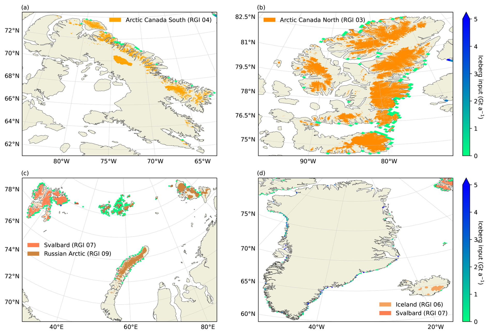
Figure A2 Iceberg input distribution in the halfsolid NEMO run setup (2010 to 2019 average). Regions shown are (a) Baffin Island, (b) Queen Elizabeth Island (CAA), (c) Barents and Kara Sea, and (d) Greenland and Iceland. In the noOGGM run setup only the icebergs around Greenland, displayed in panel (d) and derived from Bamber et al. (2018), are added to the ocean. Colored land areas indicate the named glacierized regions as recorded in the RGI.

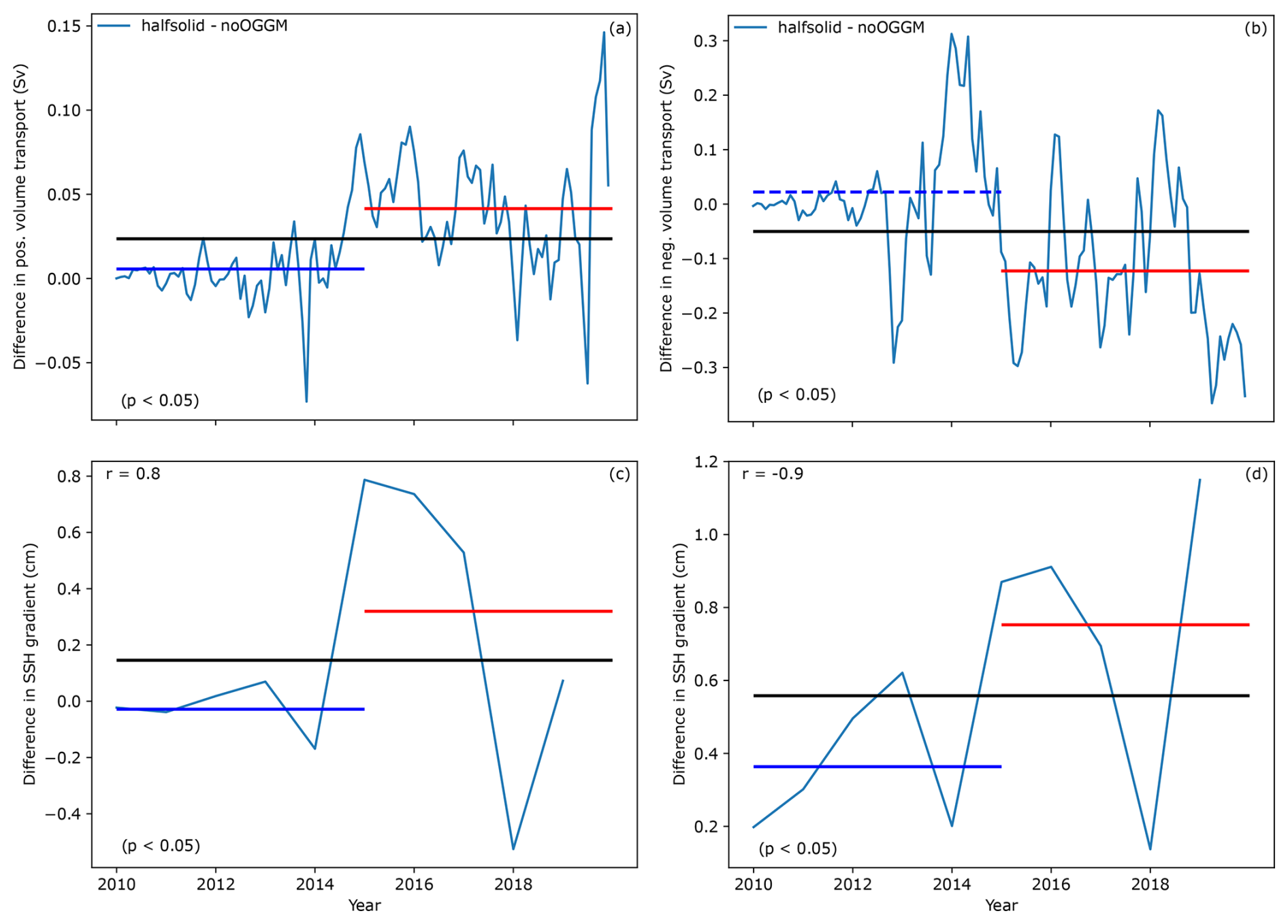
Figure A3 Differences in gyre strength and SSH gradients in Baffin Bay between the halfsolid and the noOGGM NEMO runs. (a) Northward (positive) volume transport through the eastern part of the Baffin Bay gyre (BBG) section in Fig. 3, (b) southward (negative) volume transport through western part of the BBG section, and (c) annual mean SSH gradient between the point with the highest average SSH in the eastern part of the BBG section and the point with the lowest average SSH in the center part of the section. Panel (d) is the same as (c), but for the point with the highest average SSH in the western part of the BBG section. Differences in SSH gradients are displayed as annual means for better visibility. The horizontal lines show average differences over the first (blue) and last (red) 5 years, as well as over all years (black) of the model integrations. Differences between the two NEMO runs that are statistically significant, according to Wilcoxon signed-rank tests (p<0.05), are drawn as solid lines and dashed otherwise. Values in the lower left corners show the p values of Wilcoxon signed-rank tests of differences between the differences of the first and last 5 modeled years. Values in the upper left corners of panels (c) and (d) are the correlation coefficients between annual mean northward and southward volume flux and SSH gradients from the east and west to the center of the Baffin Bay gyre.

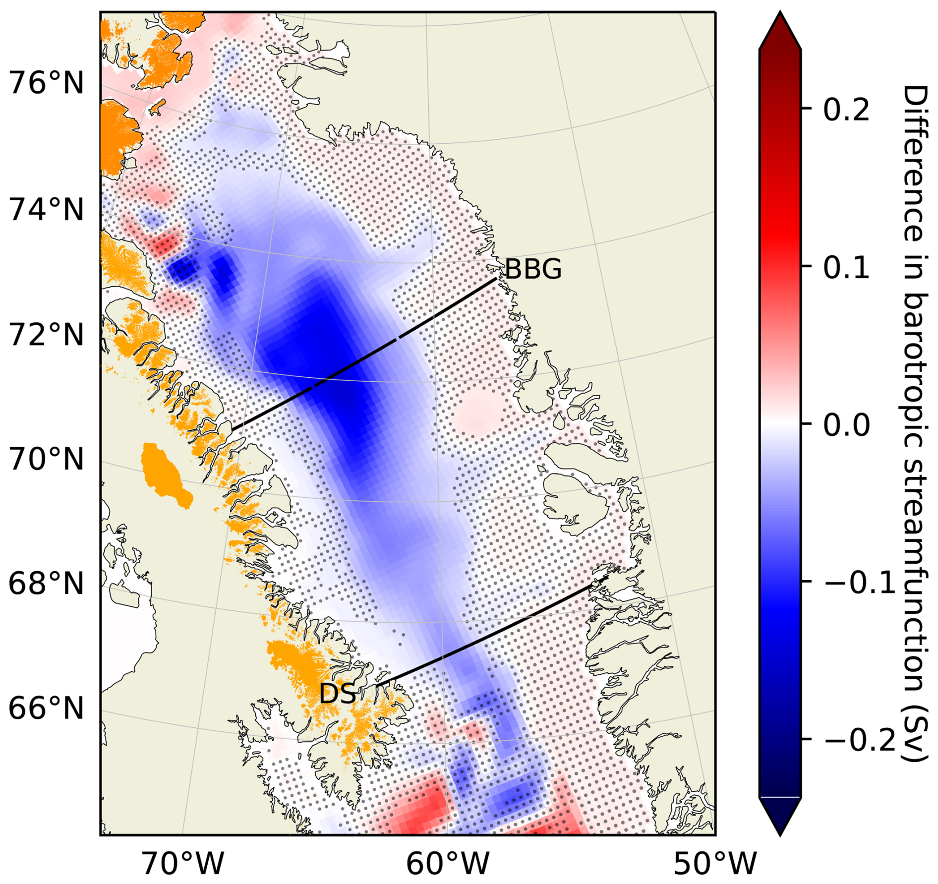
Figure A4 Difference in barotropic streamfunction between the halfsolid and noOGGM NEMO runs in the Baffin Bay area. Dots indicate differences that are not statistically significant, according to Wilcoxon signed-rank tests (p>0.05). Colored land area indicates glacierized area as recorded in the RGI.

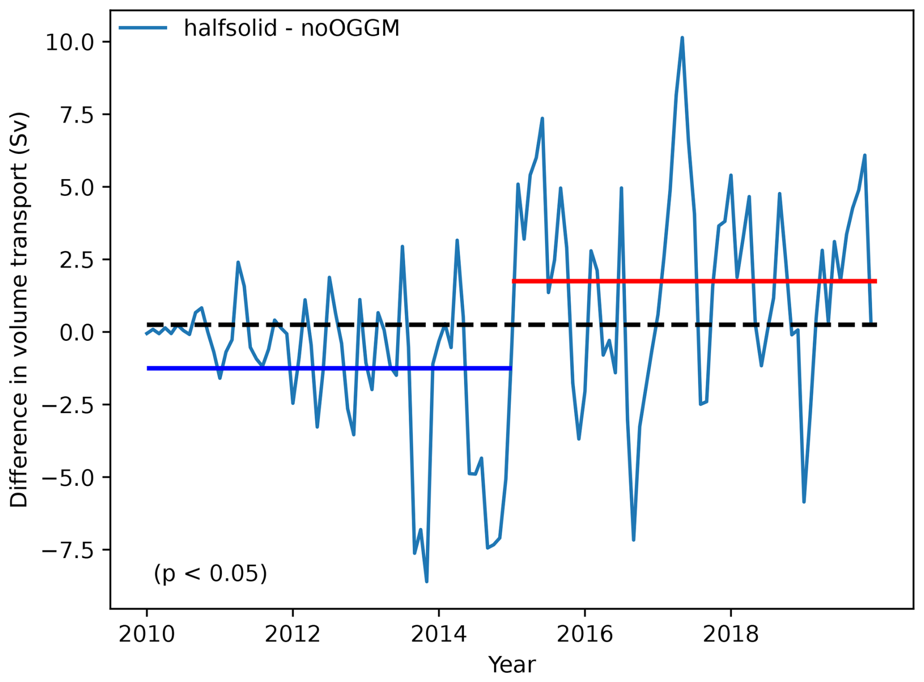
Figure A5 Differences in WGC volume transport at Cape Desolation. The horizontal line shows the average difference over the first (blue) and last (red) 5 years, as well as over all years (black) of the model integrations. Differences between the two NEMO runs that are statistically significant, according to Wilcoxon signed-rank tests (p<0.05), are drawn as solid lines and dashed otherwise. Values in the lower left corners show the p values of Wilcoxon signed-rank tests of differences between the first and last 5 modeled years.

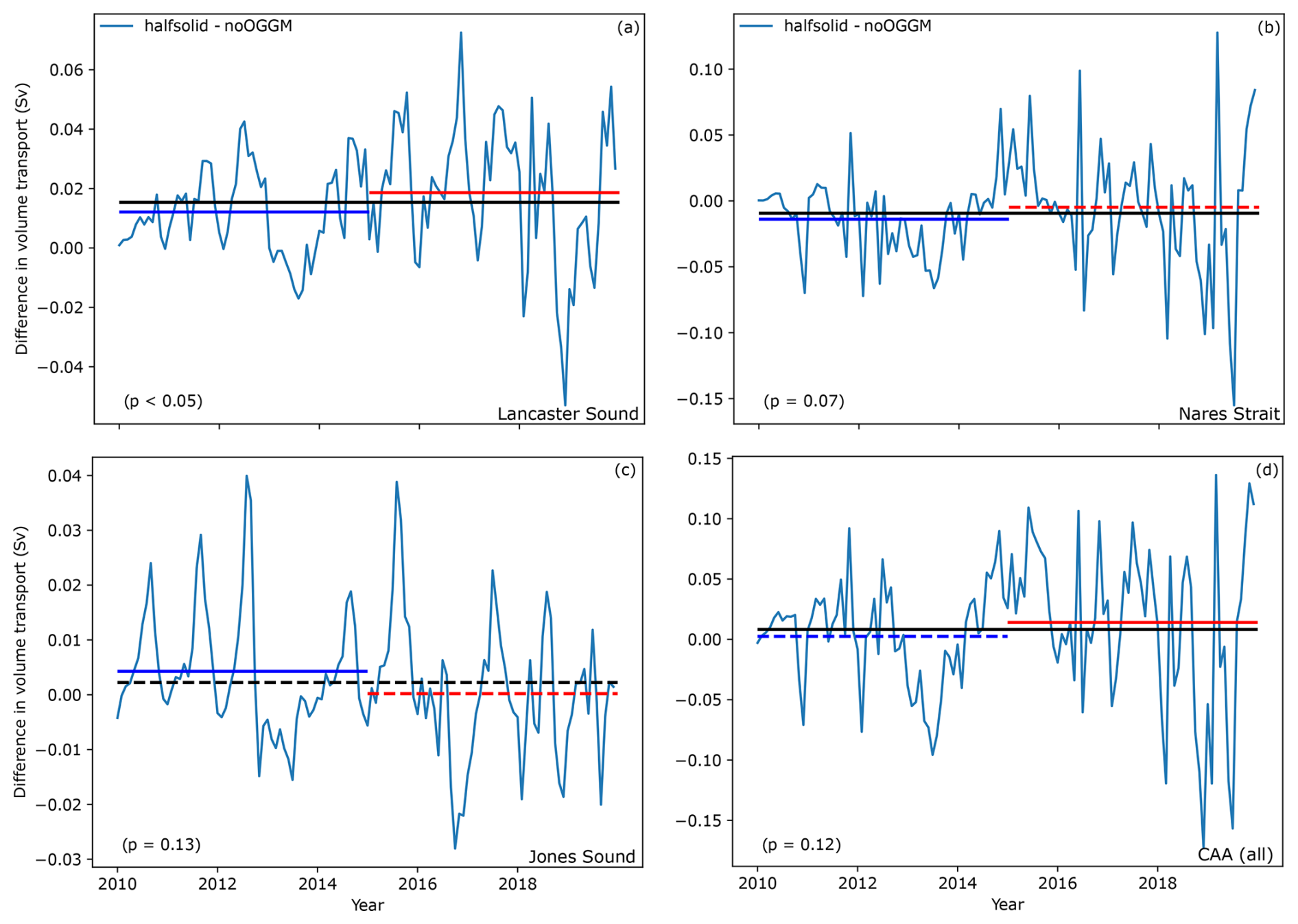
Figure A6 Differences in volume transport through the three main ocean pathways connecting the CAA and Baffin Bay (a–c) and (d) the volume transport through all three. Note that volume flux northward through the CAA is defined as positive. The horizontal lines show average differences over the first (blue) and last (red) 5 years, as well as over all years (black) of the model integrations. Differences between the two NEMO runs that are statistically significant, according to Wilcoxon signed-rank tests (p<0.05), are drawn as solid lines and dashed otherwise. Values in the lower left corners show the p values of Wilcoxon signed-rank tests of differences between the first and last 5 modeled years.

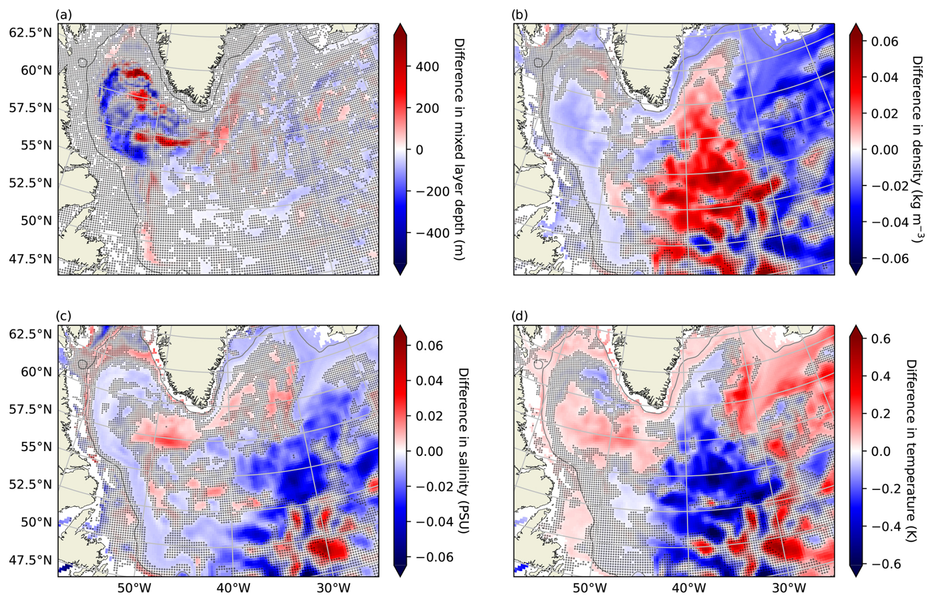
Figure A7 Difference in (a) January–February–March mixed layer depth, (b) density, (c) salinity, and (d) potential temperature averaged over 200–600 m water depth between the halfsolid and noOGGM NEMO runs in the subpolar gyre region. Dots indicate differences that are not statistically significant, according to Wilcoxon signed-rank tests (p>0.05). Gray lines show the low-pass-filtered 600 m bathymetry contours.

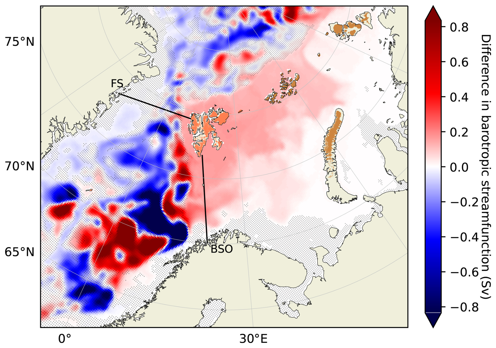
Figure A8 Difference in barotropic streamfunction between the halfsolid and noOGGM NEMO runs in the Barents Sea and Nordic Seas area. Dots indicate differences that are not statistically significant, according to Wilcoxon signed-rank tests (p>0.05). Colored land area indicates glacierized area as recorded in the RGI.

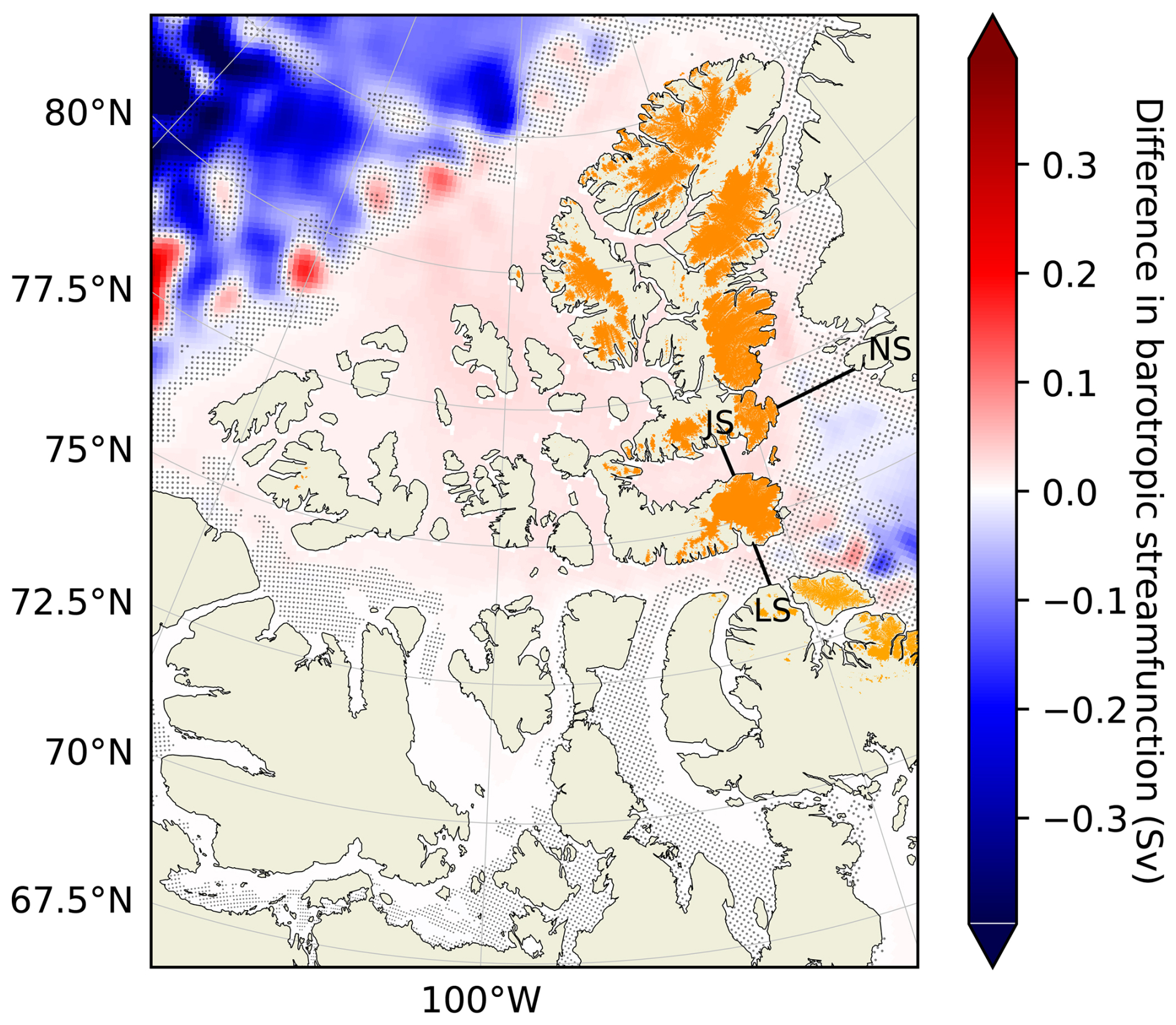
Figure A9 Difference in barotropic streamfunction between the halfsolid and noOGGM NEMO runs in the CAA region. Dots indicate differences that are not statistically significant, according to Wilcoxon signed-rank tests (p>0.05). Colored land area indicates glacierized area as recorded in the RGI.

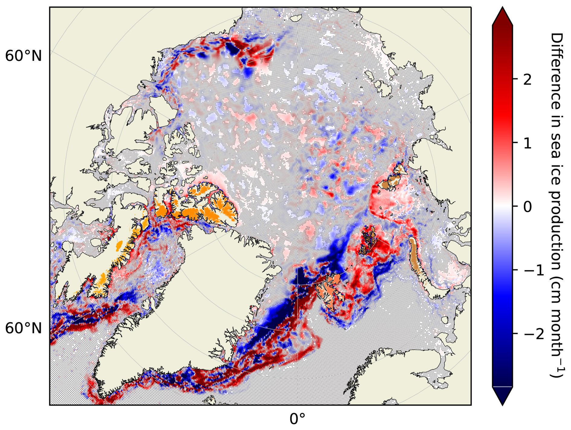
Figure A10 Difference in monthly sea ice production between the halfsolid and noOGGM NEMO runs. Dots indicate differences that are not statistically significant, according to Wilcoxon signed-rank tests (p>0.05). Colored land area indicates glacierized area as recorded in the RGI.

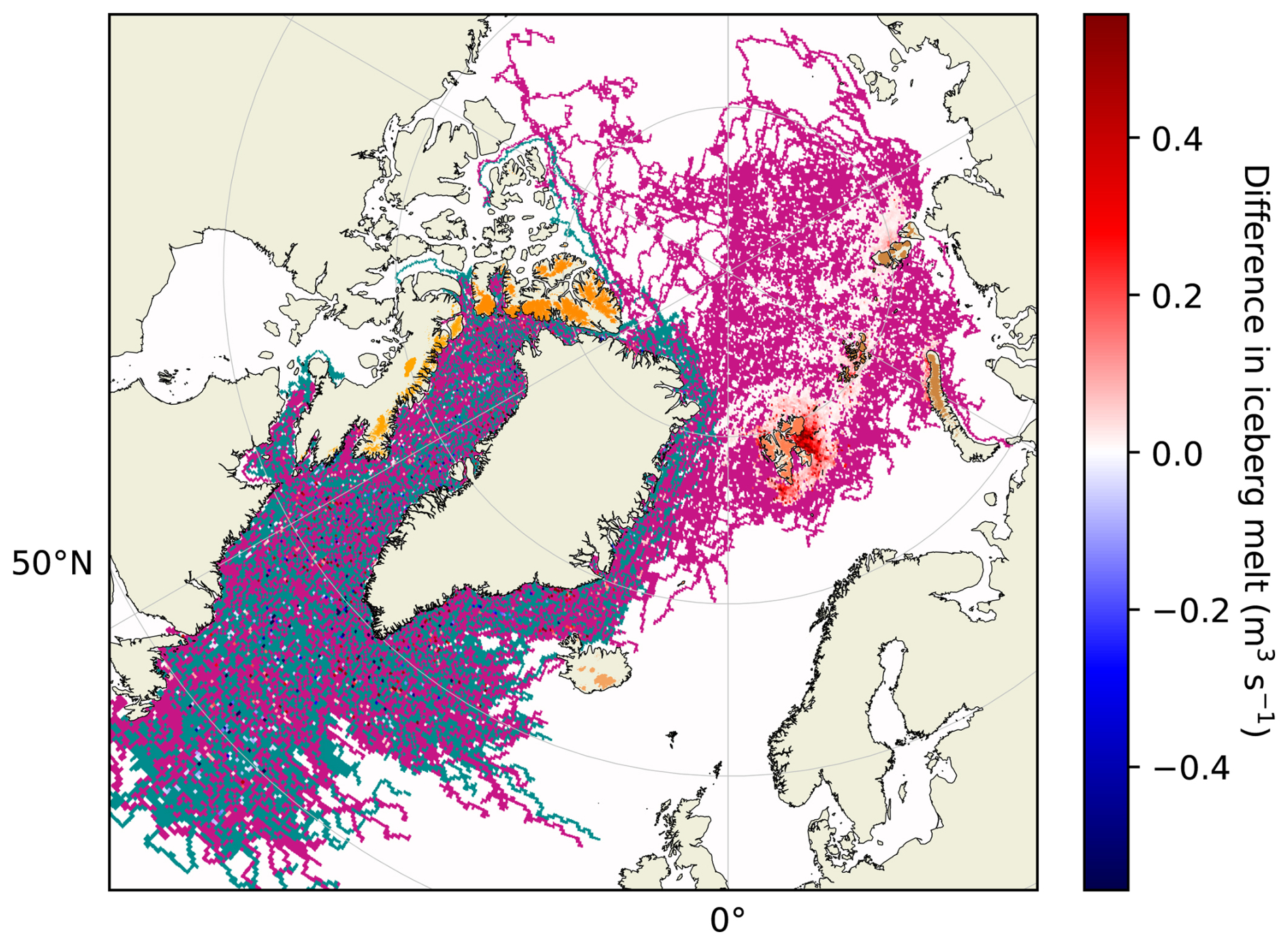
Figure A11 Difference in iceberg melt between the halfsolid and noOGGM NEMO runs. For visibility, purple and cyan areas indicate positive and negative differences that are not statistically significant according to Wilcoxon signed-rank tests (p>0.05). Colored land area indicates glacierized area as recorded in the RGI.

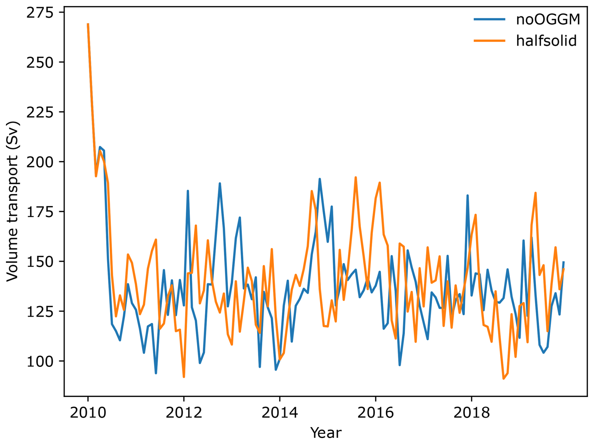
Figure A12 Positive (northward) transport across a section along 47° N (48.5 to −11.5° W) in the halfsolid and noOGGM NEMO runs. This transport feature mostly consists of the North Atlantic Current.