the Creative Commons Attribution 4.0 License.
the Creative Commons Attribution 4.0 License.
 | 15 Jul 2024
A missing link in the carbon cycle: phytoplankton light absorption under RCP emission scenarios
Philip B. Holden
Frank Lunkeit
Inga Hense
Marine biota and biogeophysical mechanisms, such as phytoplankton light absorption, have attracted increasing attention in recent climate studies. Under global warming, the influence of phytoplankton on the climate system is expected to change. Previous studies analyzed the impact of phytoplankton light absorption under prescribed future atmospheric CO2 concentrations. However, the role of this biogeophysical mechanism under freely evolving atmospheric CO2 concentration and future CO2 emissions remains unknown. To shed light on this research gap, we perform simulations with the EcoGEnIE Earth system model (ESM) and prescribe CO2 emissions out to the year 2500 following the four Extended Concentration Pathway (ECP) scenarios, which for practical purposes we call Representative Concentration Pathway (RCP) scenarios. Under all RCP scenarios, our results indicate that phytoplankton light absorption leads to a shallower remineralization of organic matter and a reduced export efficiency, weakening the biological carbon pump. In contrast, this biogeophysical mechanism increases the surface chlorophyll by ∼ 2 %, the sea surface temperature (SST) by 0.2 to 0.6 °C, the atmospheric CO2 concentrations by 8 %–20 % and the atmospheric temperature by 0.3 to 0.9 °C. Under the RCP2.6, RCP4.5 and RCP6.0 scenarios, the magnitude of changes due to phytoplankton light absorption is similar. However, under the RCP8.5 scenario, the changes in the climate system are less pronounced due to decreasing ecosystem productivity as temperature increases, highlighting a reduced effect of phytoplankton light absorption under strong warming. Additionally, this work highlights the major role of phytoplankton light absorption on the climate system, suggesting highly uncertain feedbacks on the carbon cycle with uncertainties that may be in the range of those known from the land biota.
- Article
(3936 KB) - Full-text XML
- BibTeX
- EndNote


Under anthropogenic climate change, observations indicate that the future changes of phytoplankton biomass and net primary production are highly uncertain. For instance, satellite observations demonstrate that low-latitude oceans have become greener due to climate change between 2002–2022 (Cael et al., 2023). In contrast, oceanographic measurements from 1890 to 2010 reveal that chlorophyll concentrations have declined over more than 62 % of the ocean surface (Boyce et al., 2014). Additionally, Polovina et al. (2008) indicate that, between 1998 and 2006, areas with low surface chlorophyll have expanded by 15 % on a global scale, although their results might not be exclusively attributed to climate change due to their short time series (Henson et al., 2010; Schlunegger et al., 2020). Using an ocean color database spanning 6 years, McClain et al. (2004) show that the oligotrophic waters expand in the Northern Hemisphere, while the expansion in the Southern Hemisphere is much weaker. Complementing these observations, modeling studies have also investigated the future changes in net primary production due to anthropogenic warming. For instance, on a global scale, a CMIP6 model ensemble study indicates a decrease in depth-integrated net primary production of 2.99 ± 9.11 % by the end of the 21st century under the high-emission scenario SSP5-8.5 (Kwiatkowski et al., 2020). However, this estimate is rather imprecise due to incomplete understanding and insufficient observational constraints; thus the projections of net primary production changes show large uncertainties (Tagliabue et al., 2021). On a regional scale, projected changes in primary production are also uncertain. For instance, in the Mediterranean Sea, Richon et al. (2019) show a decline in net primary production of 10 % in the 2090s under the high-emission SRES-A2 scenario. However, in the same basin, Reale et al. (2022) demonstrate that, under the RCP4.5 and RCP8.5 scenarios, the net primary production increase is greater than 10 gC m−2 yr−1 by the end of the 21st century. These conflicting results come from the different parameterizations adopted which exert differing influences of temperatures on simulated net primary production. These changes in primary production, phytoplankton abundance, distribution and biogeography consequently have an impact on the role of phytoplankton light absorption.
Different modeling studies investigate the effect of phytoplankton light absorption on the oceanic temperature under global warming. It is suggested that the decrease in phytoplankton abundance will increase ocean clarity and lead to a lower biological increase in sea surface temperature (SST). A reduction in phytoplankton-induced oceanic warming could thus counteract in part the warming associated with climate change (Patara et al., 2012). To study the effect of phytoplankton light absorption in a warming scenario, Sonntag (2013) modified the oceanic forcing by increasing the sea surface temperature for the whole model domain by 3 °C. Taking into account phytoplankton light absorption, surface phytoplankton concentrations are enhanced and the maximum SST increase is 0.4 °C compared to a present-day scenario (Sonntag, 2013). Furthermore, Paulsen (2018) uses an Earth system model (ESM) of high complexity to perform simulations under a transient increase of 1 % in atmospheric CO2 per year. With phytoplankton light absorption, Paulsen (2018) reports a decline in chlorophyll concentrations in the upwelling regions due to a reduced upwelling strength. However, this local effect is outweighed by advective processes such as the upward transport of warmer subsurface water originating off-Equator, leading a local oceanic warming of up to 0.7 °C. Additionally, the sensitivity of the light attenuation coefficient for phytoplankton is investigated under the RCP8.5 scenario (Kvale and Meissner, 2017). Depending on the parameterization choice, the authors highlight that phytoplankton light absorption may reduce or increase net primary production between 1800 and 2100. Additionally, using a coupled ocean–atmosphere model, Park et al. (2015) focus on the Arctic region to study phytoplankton light absorption under global warming. They conduct simulations where atmospheric CO2 concentration increases by 1 % per year from the level of 1990 to double its initial concentration. The authors show that phytoplankton light absorption amplifies future Arctic warming by 20 %. All these previous studies have demonstrated that phytoplankton light absorption affects the future climate projections, but, to this day, this biogeophysical mechanism is missing from 50 % of the CMIP6 models (Pellerin et al., 2020).
To date, the impact of phytoplankton light absorption on oceanic temperature under oceanic warming (Sonntag, 2013), constant atmospheric CO2 concentration (Patara et al., 2012) and prescribed rising atmospheric CO2 concentrations (Park et al., 2015; Kvale and Meissner, 2017; Paulsen, 2018) has been investigated. However, Asselot et al. (2022) study how atmospheric temperature is affected by phytoplankton light absorption. To do so, the authors compare the changes in air–sea heat versus air–sea CO2 exchange due to this biogeophysical mechanism. They conclude that phytoplankton light absorption mainly affects the climate system via air–sea CO2 exchange. Therefore, prescribing atmospheric CO2 concentrations for global warming simulations blurs the real effect of this biogeophysical mechanism. The purpose of this study is to better understand how phytoplankton light absorption will be affected by anthropogenic climate change via changes in phytoplankton biomass and distribution. To address this question, we performed simulations with and without phytoplankton light absorption in experiments with prescribed atmospheric CO2 emissions. We are interested in long-term climate effects, so we applied the intermediate-complexity Earth system model EcoGEnIE (Ward et al., 2018). We force the model with atmospheric CO2 emissions out to 2500 following the four extended Representative Concentration Pathway (RCP) scenarios used by the Intergovernmental Panel on Climate Change (IPCC) for their Fifth Assessment Report (Moss et al., 2010).
The Earth System model (ESM) used in this study is called EcoGEnIE (Ward et al., 2018) and is a coupling between a new ecosystem component (ECOGEM) and cGEnIE (Ridgwell et al., 2007). EcoGEnIE is an ESM of intermediate complexity (EMIC) (Claussen et al., 2002), and, due to the limitations of such a model, in particular its low resolution, we focus on the quantification of the large-scale impacts of phytoplankton light absorption. We chose to conduct our study with an EMIC because we are interested in the effect on a particular climate mechanism (e.g., phytoplankton light absorption), and it would have been difficult to isolate this effect with an ESM of high complexity due to numerous climate feedbacks implemented in high-complexity ESMs. For instance, in our model setup, the wind is prescribed and does not change between simulations. Consequently, the effect of wind on ocean circulation is unchanged between the simulations and through time. Moreover, cGEnIE is widely used to study past climate systems and the carbon cycle over geological timescales (Gibbs et al., 2016; Meyer et al., 2016; Greene et al., 2019; Stockey et al., 2021). EcoGEnIE was already used to analyze the role of marine phytoplankton in the warm early Eocene period (Wilson et al., 2018) and to explore the relationships between plankton size, trophic complexity and the availability of phosphorus during the late Cryogenian (Reinhard et al., 2020). We use the same configuration as described in Asselot et al. (2021). This model contains components that represent climate processes, including ocean dynamics, marine biogeochemistry, marine ecosystem, atmospheric circulation and sea-ice dynamics (Fig. 1). We do not consider a dynamical land scheme, and we neglect the terrestrial carbon cycle. For this study, we modify the ecosystem component and the oceanic component to implement phytoplankton light absorption.
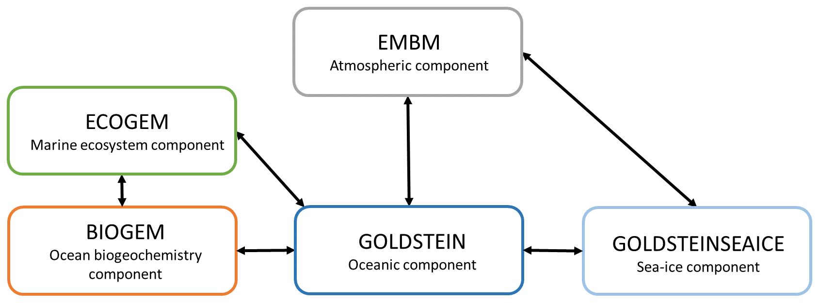
Figure 1Sketch representing the different components of the EcoGEnIE model. Black arrows represent the links between the different components. GEnIE is controlled by a bespoke coupling manager which was developed for user-friendly modularity and flexibility so that, for instance, the EMBM atmosphere can be replaced with a fully dynamic 3D atmosphere PLASIM (Holden et al., 2016) via a single switch in the model configuration file. Figure from Asselot et al. (2022).
2.1 Ocean, atmosphere and sea-ice representation
The oceanic component is a 3D frictional geostrophic oceanic component (GOLDSTEIN) that calculates the horizontal and vertical redistribution of heat, salinity and biogeochemical elements (Edwards and Marsh, 2005). The horizontal grid (36 × 36) is uniform in longitude (10° resolution) and uniform in sine latitude, giving ∼ 3.2° latitudinal increments at the Equator increasing to 19.2° in the polar regions. This horizontal grid has been employed as the standard resolution to study the global carbon cycle (Cameron et al., 2005). Furthermore, we consider 32 vertical oceanic layers, increasing logarithmically from 29.38 m for the surface layer to 456.56 m for the deepest layer. The model underestimates the upwelling in the northeastern Atlantic, in the Arabian Sea and in polar regions (Ward et al., 2018). In contrast, Ridgwell et al. (2007) indicate that the low-latitude upwelling in the western equatorial Pacific and equatorial Indian Ocean gives an excess of phosphate of 0.5 µmol kg−1 compared to observations (Conkright, 2002).
The atmospheric component is an energy moisture balance model (EMBM), which is closely based on the UVic Earth system model (Weaver et al., 2001). It is a 2D slab layer of the atmosphere where atmospheric temperature and specific humidity are the prognostic variables. Heat and moisture are horizontally transported by winds and mixing. The incoming shortwave radiation at the top of the atmosphere depends on the planetary albedo, which varies as a function of latitude and time of year to account for the effects of changes in solar zenith angle. The net longwave radiation represents ∼ 45 % of the total atmospheric energy balance, while net shortwave radiation represents ∼ 25 %. The radiative forcing associated with changes in atmospheric CO2 concentrations is considered in the calculation of outgoing planetary longwave radiation (QPLW). Higher atmospheric CO2 concentration leads to higher amounts of QPLW being trapped in the atmosphere. Furthermore, the parameterization for QPLW is taken from Thompson and Warren (1982) and depends on the surface relative humidity and atmospheric temperature through a logarithmic dependency. Precipitation instantaneously removes all moisture corresponding to the excess above a relative humidity threshold. Wind velocities are prescribed following the annual average data of Trenberth (1989), and a constant and dimensionless land surface drag coefficient is set to (Weaver et al., 2001).
The sea-ice component (GOLDSTEINSEAICE) solves the fraction of the ocean surface covered by ice within a grid cell and computes the average sea-ice thickness (Edwards and Marsh, 2005). A diagnostic equation is solved for the ice surface temperature. The growth or decay of sea ice depends on the net heat flux into the ice (Hibler, 1979; Semtner, 1976). Sea-ice dynamics consist of advection by surface currents and diffusion. The sea-ice component acts as a coupling module between the ocean and the atmosphere, where heat and freshwater are exchanged and conserved between these three modules.
2.2 Ocean biogeochemistry component
The biogeochemical module (BIOGEM) represents the transformation and spatial redistribution of biogeochemical tracers (Ridgwell et al., 2007). The state variables are inorganic nutrients and organic matter. Organic matter is partitioned into dissolved and particulate organic matter (DOM and POM). The model includes iron (Fe) and phosphate (PO4) as limiting nutrients. Similarly to Asselot et al. (2021), we do not explicitly consider nitrate (NO) but approximate it through the N : P Redfield ratio of 16 : 1 (Ridgwell et al., 2007). Furthermore, BIOGEM calculates the air–sea CO2 and O2 exchange. These fluxes depend on the gas transfer velocity, the water density, the concentration of dissolved gas in the ocean surface, the solubility coefficient calculated from Wanninkhof (1992), the concentration of gas in the atmosphere and the fraction of the ocean covered by sea ice (Ridgwell et al., 2007).
2.3 Ecosystem community component
The marine ecosystem component (ECOGEM) represents the marine plankton community and associated interactions within the ecosystem (Ward et al., 2018). The biological uptake in ECOGEM is limited by light, temperature and nutrient availability. Phytoplankton are allowed to flexibly take up nutrients according to availability. The production of dead organic matter is a function of mortality and messy feeding. The surface production is then distributed along the water column as a depth-dependent flux. To achieve this, the flux is partitioned between POM, of which on average 70 % is remineralized below the euphotic layer (0–221.84 m), and DOM, which is predominantly remineralized within this layer. In ECOGEM, the sinking speeds of organic matter are constant. The model assumes that photosynthesis is a Poisson function of irradiance and that phytoplankton growth is limited by this function (Geider et al., 1998; Moore et al., 2001). The phytoplankton growth model requires NO to simulate chlorophyll synthesis, but we do not consider this nutrient in our study. As a consequence, the nitrate biomass is equal to the phosphate biomass multiplied by the standard Redfield ratio of 16 (Ward et al., 2018). Nutrient uptake is a Michaelis–Menten function, and phytoplankton growth is limited by a minimum function of internal nutrient status. Plankton biomass and organic matter are subject to processes such as resource competition and grazing before being passed to DOM and POM. The ecosystem is divided into different plankton functional types (PFTs) with specific traits. Each PFT can be subdivided into size classes with specific size-dependent traits. However, we incorporate only two PFTs: one phytoplankton and one zooplankton group. We consider only one phytoplankton and one zooplankton class size, following the low-ecosystem-complexity model of Asselot et al. (2021), noting that Asselot et al. (2021) found that the climate impact of changing ecosystem complexity was negligible compared to that from phytoplankton light absorption. Phytoplankton is characterized by nutrient uptake and photosynthesis, whereas zooplankton is characterized by predation traits. Zooplankton grazing depends on the concentration of prey biomass and prey size, with zooplankton predominantly grazing on prey that is 10 times smaller than themselves. The model regards inorganic resources (DIC, PO4 and Fe), plankton biomass and organic matter (POM and DOM) as state variables. Living matter is not subject to ocean transport. Communication between biological communities only occurs through the advection and diffusion of inorganic and non-living organic matter. This approximation is justified by the coarse model resolution (∼ 1000 km) and limited transport range of living matter, so the rate of transport between grid cells is slow in relation to the net growth rates of the plankton community (Ward et al., 2018). ECOGEM considers a dynamic photoacclimation (Geider et al., 1998) where the chlorophyll-to-carbon ratio is regulated as the cell attempts to balance the rate of light capture by chlorophyll with the maximum potential rate of carbon fixation. Phytoplankton biomass can only be lost via grazing and mortality. Plankton mortality is reduced at very low biomass such that plankton cannot become extinct. The production of alkalinity is coupled to phytoplankton uptake of phosphate via a fixed linear ratio, meaning that alkalinity increases while phosphate is consumed. The exports of calcium carbonate (CaCO3) and alkalinity are scaled to the export of POC via a spatially uniform value which is modified by a thermodynamically based relationship with the calcite saturation state. The dissolution of CaCO3 below the surface is treated similarly to that of POM.
2.4 Temperature limitation
Metabolic processes of photosynthesis, nutrient uptake and zooplankton predation are all driven by the same exponential temperature limitation term (Ward et al., 2018). The temperature limitation scheme is given by Eq. (1):
where γT is the temperature limitation, A is the temperature sensitivity (0.05 °C−1), T is the sea surface temperature and Tref is the reference temperature. A reference temperature of 20 °C is used because most experimentally determined metabolic rates are made at this temperature (Behrenfeld and Falkowski, 1997; Goldman, 1977; Rhee and Gotham, 1981). Photosynthesis is light-limited, which results in a sub-exponential growth rate, while competing effects of nutrient demand and zooplankton predation increase exponentially and together progressively limit net productivity as temperatures increase. We note that temperature dependence may be complicated by co-varying factors such as nutrient availability, leading to disproportionate effects depending on location. To explore these dependencies, chlorophyll and nutrient density are plotted against SST in Figs. A1 and A2 in Appendix A, respectively, with data separated into binned subsets with different nutrient density. When nutrient density is low (<0.017 mmol m−3), 30 % of the variance in chlorophyll is explained by temperature, with a negligible contribution of co-varying nutrients (only 7 % of nutrient variance can be explained by SST in this bin). In contrast, under high nutrient concentrations (>0.1 mmol m−3), while 51 % of the variance in chlorophyll can be explained by temperature, as much as 41 % of this could be explained by the co-variance in nutrients with temperature. In summary, chlorophyll is limited by increasing temperature through both increased nutrient demand and zooplankton grazing and through reduced nutrient availability, likely, at least in part, driven by the increasing nutrient demand.
2.5 Phytoplankton light absorption
In the original model version (Ward et al., 2018), light was only absorbed by phytoplankton. Following Asselot et al. (2021), a new light scheme is implemented where the absorbed light by phytoplankton is converted into heat and is able to affect the oceanic temperature. In the current model configuration, the incoming shortwave radiation varies seasonally. Moreover, the light level is calculated as the mean level of photosynthetically available radiation within each oceanic layer. The light penetrates until the sixth oceanic layer of the model (221.84 m), representing the base of the euphotic zone. The maximum light absorption occurs in the surface layer, while the minimum absorption happens in the sixth layer. The propagation of light within the ocean is limited by pure water and chlorophyll cells (Ward et al., 2018). The vertical light attenuation scheme is given by Eq. (2):
where I(z) is the radiation at depth z, I0 is the radiation at the surface of the ocean, kw is the light absorption by clear water (0.04 m−1), kChl is the light absorption by chlorophyll (0.03 m−1 (mg Chl)−1) and Chl(z) is the chlorophyll concentration at depth z. The values for kw and kChl are taken from Ward et al. (2018). The parameter I0 is negative in the model because it is a downward flux from the sun to the surface of the ocean. Phytoplankton changes the optical properties of the ocean through phytoplankton light absorption, causing radiative heating and changing the heat distribution in the water column (e.g., Wetzel et al., 2006; Anderson et al., 2007; Sonntag, 2013). We implement phytoplankton light absorption into the model (Eq. 3) following the scheme of Hense (2007) and Patara et al. (2012):
denotes the water temperature change only associated with radiative heating, cp is the specific heat capacity of water, ρ is the ocean density, I is the solar radiation incident at the ocean surface and z is depth. We assume that the whole light absorption heats the water (Lewis et al., 1983).
2.6 The Representative Concentration Pathway scenarios
The RCP scenarios include the temporal evolution of greenhouse gas emissions into the atmosphere (Moss et al., 2010). Originally, there were four RCP scenarios, namely RCP2.6, RCP4.5, RCP6.0 and RCP8.5 (Fig. 2), labeled after a net enhancement of radiative forcing at the beginning of the 22nd century (2.6, 4.5, 6.0 and 8.5 W m−2, respectively). These scenarios are consistent with socio-economic assumptions and associated greenhouse gas emissions. They comprise a stringent mitigation scenario (RCP2.6), two intermediate scenarios (RCP4.5 and RCP6.0) and a high greenhouse gas emission scenario (RCP8.5). The RCP scenarios only span the 2005–2100 period, but this study is conducted on a multi-century timescale to understand the long-term climate response. As a consequence, our study requires data beyond 2100. We therefore use the Extended Concentration Pathways (ECPs) designed by stakeholders and scientific groups and spanning the 2100–2500 period (Meinshausen et al., 2011). Similarly to RCP2.6, ECP2.6 represents a strong mitigation scenario including negative CO2 emissions from 2100 to 2500. For ECP4.5 and ECP6.0, the atmospheric CO2 emissions start to decrease in the 21st century, while for ECP8.5 this decrease happens at the end of the 22nd century. For practical purposes, here, referring to the RCP scenarios indicates the period between 1765 and 2500. We consider a multi-century timescale to evaluate the long-term influence of anthropogenic CO2 emissions. Even if these emissions cease or are reduced by 2100, their influence will be echoed for centuries.
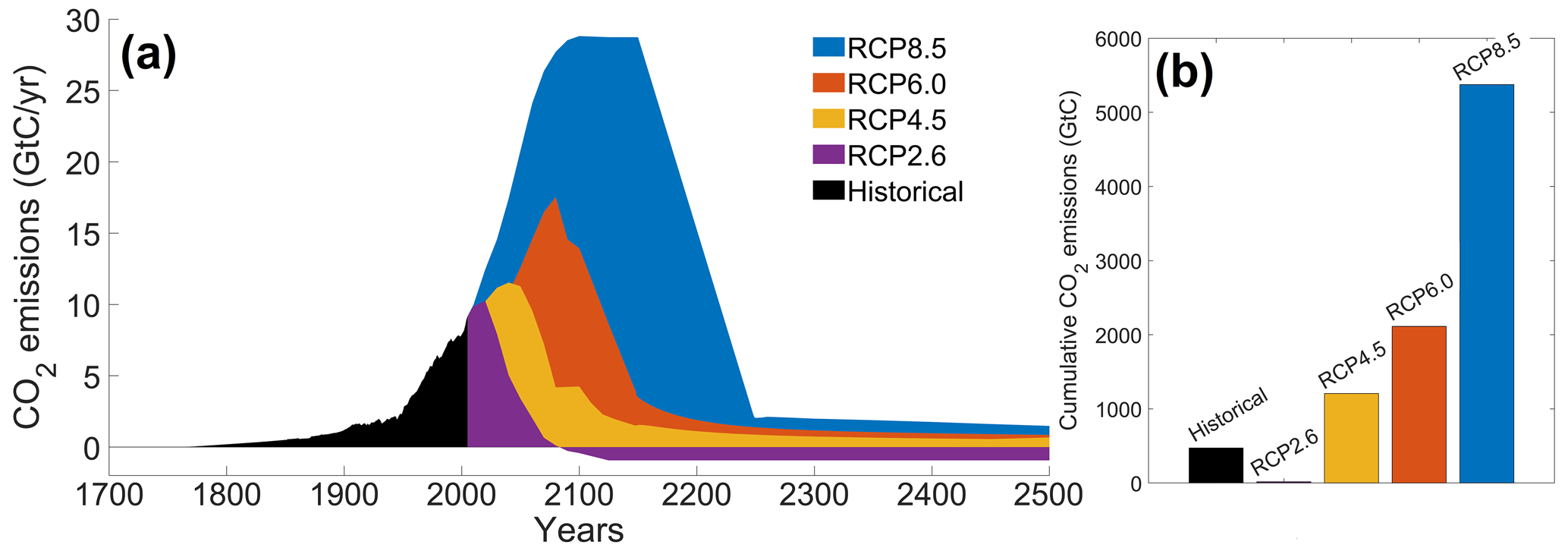
Figure 2Atmospheric CO2 emissions following the RCP scenarios. (a) Historical emissions and scenarios of future CO2 emissions over time (GtC yr−1). (b) Cumulative CO2 emissions for the different scenarios (GtC). The historical emissions represent the cumulative CO2 emissions from 1765 to 2005. The RCP scenarios represent the cumulative CO2 emissions between 2006 and 2500. The color-coding between the two panels is identical.
2.7 Model setup and simulations
We use the same model setup and parameterization as described in Asselot et al. (2021), with 32 oceanic vertical layers, net primary production allowed until the sixth vertical layer (221.84 m deep) and incoming shortwave radiation varying seasonally. The ecosystem community is consistent with the community described in Asselot et al. (2021), with one phytoplankton group and one zooplankton group (Table B1 in Appendix B). Firstly, we run a 10 000-year spin-up with only BIOGEM to achieve a realistic distribution of nutrients. The spin-up is run with a constant pre-industrial atmospheric CO2 concentration of 278 ppm. Secondly, ECOGEM is switched on, and the simulations are run for 736 years, representing the period between 1765 and 2500 (Meinshausen et al., 2011). Switching on ECOGEM has an impact on the biogeochemistry via a different uptake of nutrients and carbon. However, we are interested in the effect of light absorption by phytoplankton relative to simulations without light absorption, and our experimental results are differences between two otherwise identical simulations; the altered atmospheric CO2 and subsequent long-term drift in the carbon cycle induced by ECOGEM are common to both experiments. In total we run eight simulations with historical runs between 1765–2005 followed by RCP scenarios for the period between 2006 and 2500. The simulations are run with and without phytoplankton light absorption (Table 1). For the simulations without phytoplankton light absorption kChl=0 m−1 (mg Chl)−1, meaning that light is only attenuated by kw (Eq. 2). We run the simulations with prescribed global CO2 emissions, which are the sum of the fossil, industrial and land-use-related CO2 emissions (Fig. 2). Moreover, all simulations include ECOGEM and are forced with the same constant flux of dissolved iron into the ocean surface (Mahowald et al., 2006). We compare the yearly averaged outputs of the year 2500.
Table 1Name and description of the simulations (PLA: phytoplankton light absorption).

2.8 Model inter-comparison
To validate our model setup, we compare our results with the results of an EMIC and CMIP5 inter-comparison (Zickfeld et al., 2013), which have a model setup close to our model setup. To be consistent with Zickfeld et al. (2013), we compute the surface atmospheric temperature (SAT) increase between the periods 1986–2005 and 2081–2100, without phytoplankton light absorption. Independently of the RCP scenario, Fig. 3 shows that our increases in SAT are in agreement with the global mean warming of Zickfeld et al. (2013) and lie in between the model ensemble minimum and maximum values. Thus, our model setup is suitable to study climate change.
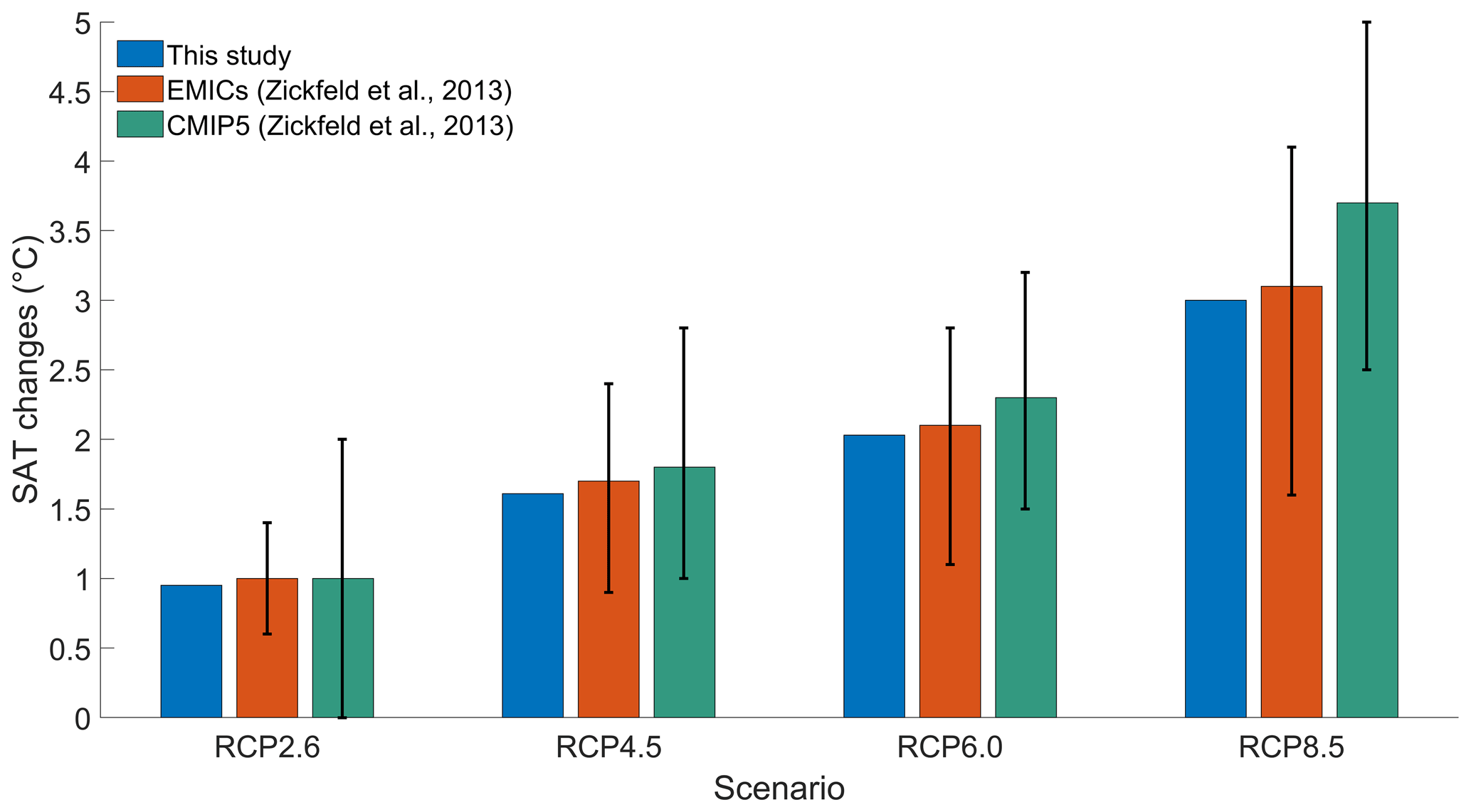
Figure 3Global mean SAT changes (°C) between the periods 1986–2005 and 2081–2100. The blue bars represent the values of our study. The orange bars represent the values of the EMIC inter-comparison of Zickfeld et al. (2013). The green bars represent the values of the CMIP5 inter-comparison of Zickfeld et al. (2013). The black vertical lines represent the minimum and maximum values from the model inter-comparison of Zickfeld et al. (2013). The SAT changes of our study come from simulations without phytoplankton light absorption.
In this section, we are interested in resolving the effects of phytoplankton light absorption and the relative differences between the simulations. Due to the limitations of such an EMIC, the absolute values are less relevant. We first look at ocean properties such as the biological pump, surface chlorophyll and SST. Secondly, we investigate the changes in atmospheric CO2 concentrations and SAT.
3.1 Oceanic properties
3.1.1 The biological carbon pump
To compare the strength of the biological carbon pump between our simulations, we consider vertical fluxes of POC in the water column. In our study, these fluxes are described by an exponential decay, which is fixed and spatially invariant. Under the RCP2.6, RCP4.5 and RCP6.0 scenarios, the POC flux decreases by 4 %–5 % when phytoplankton light absorption is activated (Table 2). For the RCP8.5 scenario, the effect is smaller, with a POC flux reduced by 1 % due to phytoplankton light absorption. In our simulations, independently of the RCP scenario, phytoplankton light absorption decreases the POC flux (Table 2), indicating that less organic matter is transported towards the bottom of the ocean. This reduced export efficiency is due to an enhanced remineralization at the ocean surface, which is driven by a higher amount of organic matter in the ocean surface. Indeed, phytoplankton light absorption increases the oceanic temperature (see below), promoting environment conditions that increase the surface remineralization (Table 2). Consequently, the nutrient concentration (Table F1 in Appendix F) and thus the net primary production in the surface ocean layer are enhanced. These results indicate that the biological pump is weaker with phytoplankton light absorption, meaning that more inorganic matter, such as nutrients, is located at the surface of the ocean (Table F1).
Table 2Comparison of global POC fluxes (1015 mol yr−1) and net primary production (GtC yr−1) in the first oceanic layer for the year 2500. Note that phytoplankton light absorption always increases the global POC flux and net primary production.

3.1.2 Surface chlorophyll
We look at the distribution of chlorophyll at the ocean surface because this climate carbon cycle variable directly affects the heat distribution along the water column through phytoplankton light absorption. On a global scale, independently of the RCP scenario, phytoplankton light absorption leads to an increase in chlorophyll at the ocean surface (Fig. 4). This increase is due to the increased global phosphate concentrations (Table F1) which are driven by a reduced export efficiency of organic matter and enhanced remineralization at the ocean surface (Table 2). For the RCP2.6, RCP4.5 and RCP6.0 scenarios, the global increase in chlorophyll is between 0.015 and 0.019 mg Chl m−3, representing an increase of 13 %–15 %. These assessments are slightly higher than previous estimates showing an increase between 4 % and 12 % (Manizza et al., 2005; Asselot et al., 2021). However, compared to our model setup, Manizza et al. (2005) use an ocean model, neglecting any interactions between the ocean and the atmosphere. Additionally, Asselot et al. (2021) do not prescribe CO2 emissions, neglecting the changes in chlorophyll due to climate change. The increase in chlorophyll for the RCP8.5 scenario is the smallest, with an increase of ∼ 0.01 mg Chl m−3, representing an increase of 8 %. The lower global increase in chlorophyll under RCP8.5 compared to the other RCP scenarios is due to the lower increase in chlorophyll in the mid-latitudes and upwelling regions (Fig. 5).

Figure 4Globally averaged surface chlorophyll (mg Chl m−3) and SST (°C) changes between the RCP scenarios in the year 2500. The values represent the difference between the simulation with minus without phytoplankton light absorption. Note that the y-axis scales are always positive, indicating that phytoplankton light absorption always leads to a global increase in surface chlorophyll and SST.
The regional patterns of surface chlorophyll changes due to phytoplankton light absorption are similar between the RCP scenarios (Fig. 5). The largest differences in chlorophyll occur at high latitudes. For example, between the simulations RCP8.5-LA and RCP8.5, the maximum increase of 0.4 mg Chl m−3 occurs in the northern polar region (Fig. 5d). This pronounced chlorophyll response in the high latitudes is likely due to enhanced light availability due to the decrease in sea ice. For instance, the global sea-ice area decreases by 13 % between RCP8.5-LA and RCP8.5, thus increasing light availability for phytoplankton growth. The upwelling and mid-latitude regions show a higher chlorophyll concentration with phytoplankton light absorption. These regional patterns are due to higher nutrient concentration at the ocean surface with phytoplankton light absorption (Table F1). This enhanced nutrient concentration is due to reduced export efficiency (Table 2) and higher remineralization at the ocean surface. The higher nutrient concentrations at the surface decrease the nutrient limitation, thus promoting a higher phytoplankton biomass at the surface. In contrast to the upwelling regions, the nutrient-limited subtropical gyres show no or small differences in surface chlorophyll concentrations.
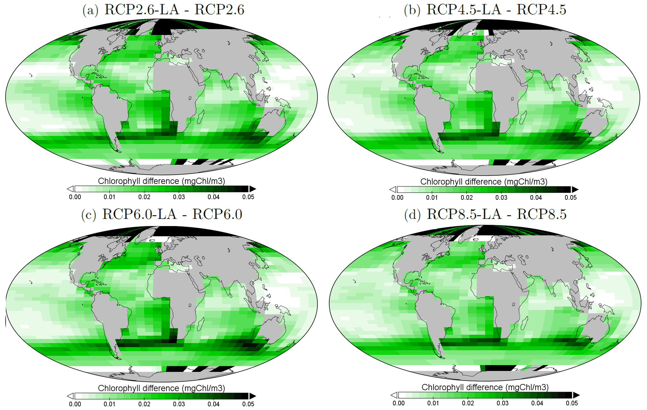
Figure 5Surface chlorophyll changes in the year 2500 (mg Chl m−3) for the different simulations. (a) Difference between RCP2.6-LA and RCP2.6. (b) Difference between RCP4.5-LA and RCP4.5. (c) Difference between RCP6.0-LA and RCP6.0. (d) Difference between RCP8.5-LA and RCP8.5. The scale and color-coding are identical in the four panels. Note that the scale is logarithmic and always positive.
3.1.3 Sea surface temperature
Our results highlight that, under the RCP2.6, RCP4.5 and RCP6.0 scenarios, phytoplankton light absorption increases the SST by ∼ 0.6 °C (Fig. 4). These assessments are higher than previous global estimates, giving a global SST increase of 0.33–0.5 °C (Wetzel et al., 2006; Patara et al., 2012; Asselot et al., 2021). This stronger increase in SST is caused by higher increases in surface chlorophyll compared to previous assessments. For the RCP8.5 scenario, phytoplankton light absorption only increases SST by 0.23 °C. This lower increase in SST is due to the lower increase in global surface chlorophyll under this scenario. Phytoplankton light absorption warms the surface of the ocean and increases the ocean heat content (Fig. C1 in Appendix C). For the scenarios RCP2.6, RCP4.5 and RCP6.0, ocean heat content in the top 2000 m increases by 16 %–79 %. For RCP8.5, this increase is strongly reduced to 0.05 %, reflecting the lower increase in global surface chlorophyll under this scenario. The regional patterns of SST changes due to phytoplankton light absorption are similar between the simulations following the RCP2.6, RCP4.5 and RCP6.0 scenarios, but the magnitude of changes differs (Fig. 6). Under these scenarios, even though the polar regions experience a high increase in chlorophyll, they also experience the lowest increase in SST. For instance, between the simulations RCP4.5-LA and RCP4.5, the minimum increase of 0.03 °C occurs in the Southern Ocean. The polar regions experience the lowest changes in SST because temperatures are buffered by latent heat through melting sea ice and remain close to freezing. In contrast, under RCP8.5, the maximum SST increase of 0.51 °C occurs in the Southern Ocean. This is due to the greatly reduced annually averaged sea ice under RCP8.5, meaning that the latent heat-buffering effect of melting and growing sea ice is weaker, allowing heating of the ocean surface. The annual ice cover in the simulation RCP8.5-LA is only 5.1×10⁶ km2 in 2500, which compares to 25.8×10⁶ km2 for RCP2.6-LA. Even in the regions where small differences in surface chlorophyll occur, such as the subtropical gyres, we find high SST increases. The differing spatial patterns between chlorophyll and SST can be explained by the fact that short-lived chlorophyll is not subject to transport, while (conserved) physical quantities, such as heat, are transported by oceanic currents. Therefore, heat is smoothly redistributed around the globe.
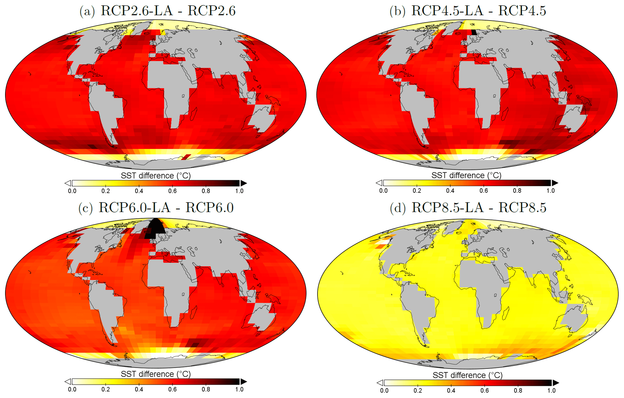
Figure 6Sea surface temperature changes (°C) between the simulations in the year 2500. (a) Difference between RCP2.6-LA and RCP2.6. (b) Difference between RCP4.5-LA and RCP4.5. (c) Difference between RCP6.0-LA and RCP6.0. (d) Difference between RCP8.5-LA and RCP8.5. The scale and color-coding are identical in the four panels. Note that the scale is always positive.
3.2 Atmospheric properties
3.2.1 Atmospheric CO2 concentration
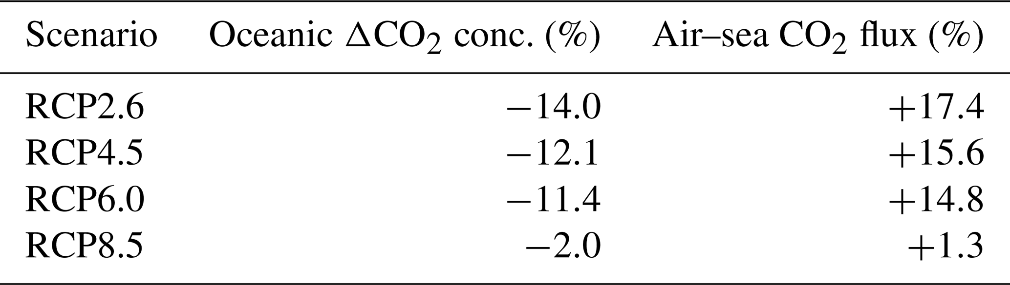
The atmospheric CO2 concentrations in our simulations do not match the atmospheric concentrations of Meinshausen et al. (2011) in 2500. This is because our version of the model, with light penetrating until the sixth oceanic layer, has been tuned to get reasonable net primary production and nutrient fields but not to get future atmospheric CO2 concentrations. As a consequence, with this configuration, the model is known to simulate low atmospheric CO2 concentrations (Asselot et al., 2021, 2022). We are interested in relative changes between our simulations rather than the absolute values, so the specifics of the background state are unlikely to affect the qualitative findings of the study, especially given that the carbon cycle response to a range of emissions is consistent with IPCC model inter-comparison projects (Fig. 3). Independently of the RCP scenario, the atmospheric CO2 concentration increases with phytoplankton light absorption (Fig. 7). For the RCP2.6, RCP4.5 and RCP6.0 scenarios, phytoplankton light absorption increases the atmospheric CO2 concentration by ∼ 20 %, while a previous study indicates an increase of 10 % (Asselot et al., 2021). However, Asselot et al. (2021) do not prescribe CO2 emissions, neglecting their effect on the atmospheric CO2 concentration. For the RCP8.5 scenario, the atmospheric CO2 concentration increases by only 8 %. This lower increase in atmospheric CO2 concentration is due to the lower decrease in oceanic CO2 content and lower increase in air–sea CO2 flux (Table D1 in Appendix D). These reduced changes between the different CO2 reservoirs are due to the lower increase in chlorophyll and SST.
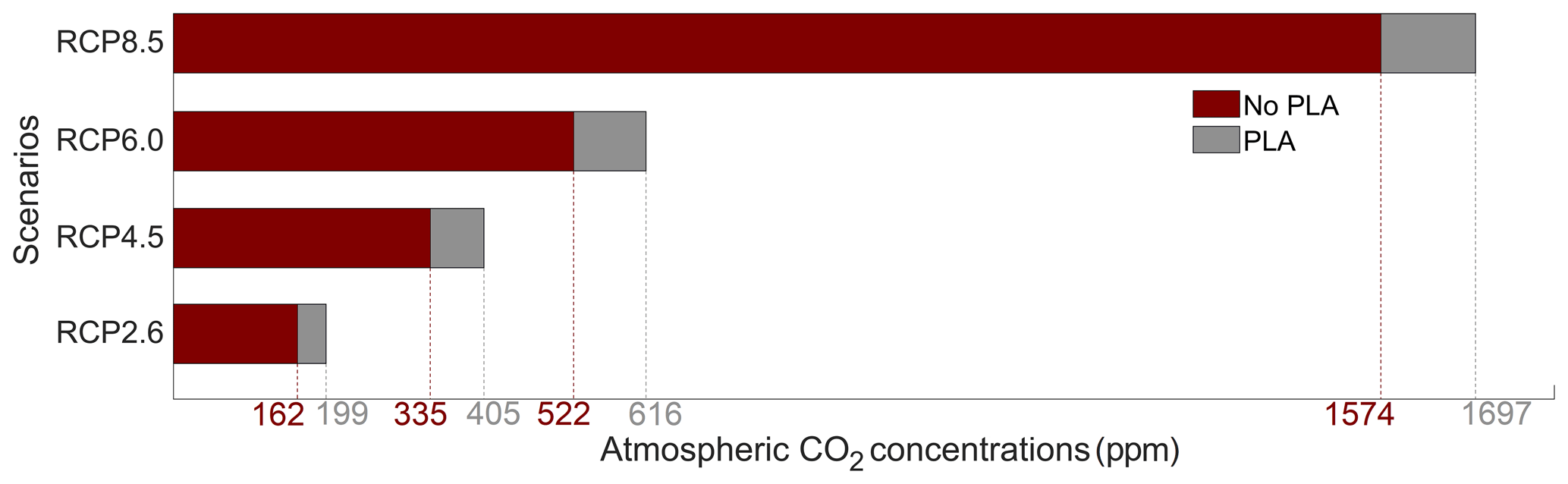
Figure 7Atmospheric CO2 concentrations (ppm) for the eight simulations in the year 2500. PLA stands for phytoplankton light absorption.
The increase in atmospheric CO2 concentrations with phytoplankton light absorption is mainly due to the higher SST decreasing CO2 solubility and oceanic CO2 content (Table D1), thus increasing the oceanic CO2 outgassing (Asselot et al., 2022). Our results indicate that the reduced solubility pump enhances the ocean-to-atmosphere CO2 flux by ∼ 10 %. In contrast, the changes in the biological and carbonate pump enhance the air–sea CO2 fluxes by < 1 %. However, the temperature dependence of solubility could not explain the changes in atmospheric CO2 concentration in steady state, suggesting that the effect is transient. For the first three RCP scenarios (but not RCP8.5), the change in atmospheric CO2 concentration driven by phytoplankton light absorption follows a roughly linear dependence on the baseline concentration for that RCP (Fig. 8). The rate of CO2 uptake is roughly proportional to baseline concentration for the first three RCP scenarios but is reduced for RCP8.5 because of the smaller effect of phytoplankton light absorption on the SST. To validate this inference, we continue our simulations for another 1000 years with no further CO2 emissions (Fig. E1 in Appendix E). These additional simulations indicate that CO2 differences decrease through time, converging towards the far smaller steady-state difference previously highlighted by Asselot et al. (2021).
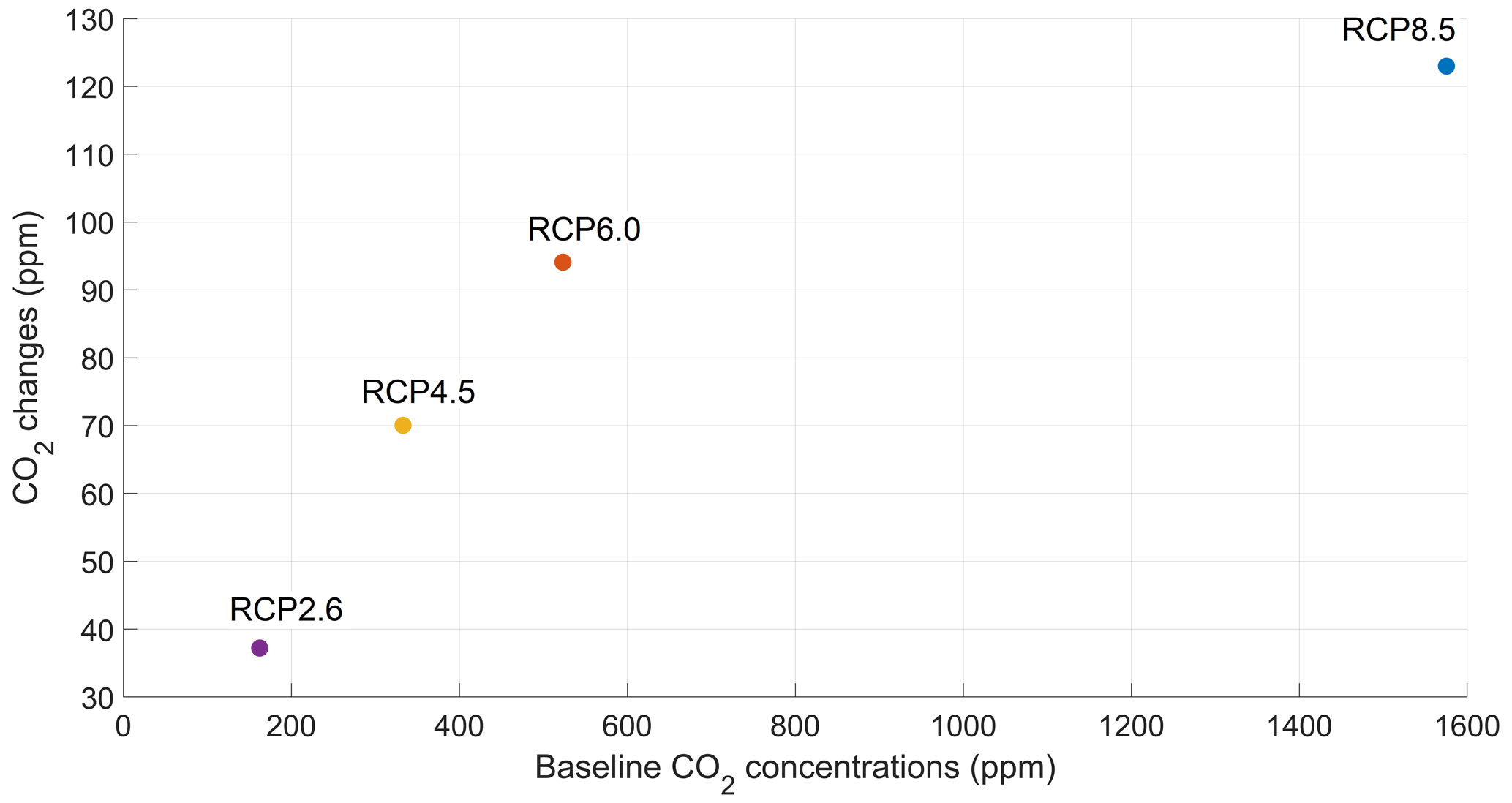
Figure 8CO2 changes (ppm) driven by phytoplankton light absorption under the four RCP scenarios in the year 2500. The x axis represents the atmospheric CO2 concentrations of the simulations without phytoplankton light absorption.
3.2.2 Surface atmospheric temperature
Due to higher greenhouse gas concentrations, the atmospheric temperature increases with phytoplankton light absorption (Fig. 9). For the RCP2.6, RCP4.5 and RCP6.0 scenarios, the global increase in SAT is ∼ 0.8 °C, which is higher than previous model estimates indicating a zonally averaged SAT increase of 0.2–0.45 °C (Shell et al., 2003; Patara et al., 2012; Asselot et al., 2021). However, compared to our model setup, Shell et al. (2003) use an uncoupled ocean–atmosphere model, neglecting any interactions between the ocean and the atmosphere. Patara et al. (2012) use a constant and prescribed atmospheric CO2 concentration for their simulations, neglecting its effect on the atmospheric temperature. Asselot et al. (2021) do not prescribe CO2 emissions, neglecting changes in the heat budget due to climate change. With a value of 0.28 °C, the increase in SAT under the RCP8.5 scenario is lower than for the other RCP scenarios. This lower value is driven by a combination of reduced SST warming and lower atmospheric CO2 concentration changes under this RCP scenario.

Figure 9Globally averaged surface atmospheric temperature (°C) changes between the RCP scenarios in the year 2500. The values represent the difference between the simulation with and without phytoplankton light absorption. Note that the y-axis scale is always positive, indicating that phytoplankton light absorption always leads to a global increase in SAT.
The regional patterns of SAT changes due to phytoplankton light absorption are similar among the RCP scenarios, but the magnitude of changes differs (Fig. 10). The polar regions experience a strong increase in SAT, with the highest values occurring in the Southern Ocean. For instance, comparing the simulations RCP4.5-LA and RCP4.5, the maximum increase of 1.6 °C occurs in the Southern Ocean (Fig. 10b). This maximum value is likely the result of reduced Antarctic sea ice (lengthening of the ice-free season) and reduction in latent heat buffering. This estimate is again higher than previous local estimates (Shell et al., 2003; Patara et al., 2012; Asselot et al., 2021) for the same reasons described above. Furthermore, around the rest of the globe, heat is redistributed smoothly in the atmosphere.

Figure 10Surface atmospheric temperature changes (°C) between the different simulations in the year 2500. (a) Difference between RCP2.6-LA and RCP2.6. (b) Difference between RCP4.5-LA and RCP4.5. (c) Difference between RCP6.0-LA and RCP6.0. (d) Difference between RCP8.5-LA and RCP8.5. The scale and color-coding are identical for the four panels. Note that the scale is always positive.
4.1 General discussion
Our results show that phytoplankton light absorption has a direct effect on oceanic temperature, consequently affecting the biogeochemical properties of the ocean. Activating phytoplankton light absorption directly increases the oceanic temperature, which reduces export efficiency of organic matter and enhanced remineralization at the ocean surface (Table 2). Consequently, the surface nutrient concentration increases (Table F1 in Appendix F), which leads to higher chlorophyll. Via the phytoplankton light absorption mechanism, this higher chlorophyll creates a feedback loop, leading to a warmer ocean. Furthermore, the higher CO2 concentration associated with phytoplankton light absorption leads to an enhanced greenhouse gas effect. As a consequence, the radiative forcing increases, warming the ocean surface as well. Under the RCP2.6, RCP4.5 and RCP6.0 scenarios, phytoplankton concentration is not strongly limited by temperature. As a result, the impact of phytoplankton light absorption on the climate system is similar between these RCP scenarios. However, under the RCP8.5 scenario, the effect of phytoplankton light absorption on the climate system is reduced. This is likely due to decreasing ecosystem productivity as temperature increases (Figs. A1 and A2), caused by exponentially increasing nutrient demand and zooplankton predation combined with sub-exponential (light-limited) increases in photosynthesis. Additionally, our results demonstrate that the increase in nutrients (Table F1) is the smallest under the RCP8.5 scenario. Consequently, fewer nutrients are available, partly explaining the reduced increase in chlorophyll under this scenario. Phytoplankton concentration is thus limited by temperature and nutrient availability, leading to a weaker difference in chlorophyll between RCP8.5-LA and RCP8.5 than between the other simulations (Fig. 4). The response of the climate system to phytoplankton light absorption is therefore weaker under the RCP8.5 scenario. Our results show that there is the potential of a tipping point, crossed in RCP8.5 in our case, at which changes in the climate system modulate the effect of phytoplankton light absorption. Our findings indicate that the effect of phytoplankton light absorption is smaller under high greenhouse gas emissions compared to reduced and intermediate greenhouse gas emissions. In agreement with Patara et al. (2012), this study indicates that a severely warmer world increases ocean clarity and slows down the warming due to phytoplankton light absorption. However, the reduced effect of phytoplankton light absorption under the RCP8.5 scenario may not be as strong if phytoplankton were able to adapt to higher temperatures in our model setup.
4.2 Limitations
For the first time, using EcoGEnIE (Ward et al., 2018), we investigate the impact of phytoplankton light absorption under prescribed CO2 emissions following the RCP scenarios on a multi-century timescale. However, our model setup has limitations that must be overcome to improve our quantitative estimates. Most notably, our version of the model must be tuned to fit the projected atmospheric CO2 concentrations under global warming scenarios. For instance, for the simulations following the RCP2.6 scenario, the final atmospheric CO2 concentrations and SSTs are lower than pre-industrial levels. This is due to the negative emissions for this scenario and the underestimation of the atmospheric CO2 concentrations with our model setup (Asselot et al., 2021, 2022). Our model setup allows light and primary production until the sixth oceanic layer, and this configuration has not been tuned to match projected atmospheric CO2 concentrations, leading to an underestimation of the latter. The lower levels under the RCP2.6 scenario compared to the pre-industrial levels are not an issue for our study because we exclusively focused on the effect of phytoplankton light absorption rather than on the differences between the simulations and the pre-industrial state. Furthermore, we switch on ECOGEM and the RCP emission forcings at the same time. We know from previous work (Asselot et al., 2021) that switching on ECOGEM decreases the atmospheric CO2 concentration; thus our simulations contain an effect of both drift and emissions. However, the drifting effect is identical between simulations and therefore balances out when comparing simulations. With our model setup we demonstrate that phytoplankton light absorption increases the local SST by 0.4–1.1 °C depending on the scenario considered. These estimates are lower than previous observations showing a local increase in SST by 0.95–4.5 °C (Kahru et al., 1993; Capone et al., 1998; Wurl et al., 2018). The difference between our estimates and observations may in part be due to the short timescales for observations, while our estimates are yearly averaged. Our results indicate a large local increase in chlorophyll in the simulations with phytoplankton light absorption, especially in the northern polar region, likely due to reduced sea ice and increased light availability. Additionally, if wind stress could evolve freely, as in classical high-complexity ESMs, we suppose that the increase in atmospheric temperature would lead to increased wind stress. As a result, upwelling dynamics would be altered. In our model setup, temperature significantly affects the concentration of our bulk phytoplankton. The temperature-dependent grazing that leads to increased grazing pressure and the temperature-dependent nutrient uptake that leads to increased nutrient limitation with increasing temperature result in a decrease in phytoplankton concentration. The response of the modeled phytoplankton might be different if we had considered different PFTs (e.g., diatoms, dinoflagellates), since their concentrations are characterized by different temperature response curves (Anderson et al., 2021). We cannot be certain that the strong phytoplankton concentration limitations in our simulations RCP8.5-LA and RCP8.5 will also occur if more PFTs are considered. Depending on the model and the region of interest, the future of net primary production is highly uncertain. For instance, using a suite of nine coupled carbon–climate ESMs under the RCP8.5 scenario, Laufkötter et al. (2015) show that net primary production may increase, remain stable or decrease under global warming. However, we note that the simulations of Laufkötter et al. (2015) only went out to 2100, not to 2500 as in our extended simulations. Our results highlight that phytoplankton light absorption increases ocean surface temperature, allowing an increase in surface remineralization and triggering an increase in nutrient concentrations. As a consequence, chlorophyll increases, allowing more heat to be trapped at the ocean surface.
4.3 Implication for Earth system models
The traditional view is that dominant carbon cycle uncertainties come from the terrestrial response to elevated atmospheric CO2 concentrations. For instance, the net land emissions from cGEnIE over the 1858–2008 period are estimated to be likely (66 % confidence) to lie in the range from 0 to 128 GtC (Holden et al., 2013). However, this work suggests that introducing biogeophysical mechanisms such as phytoplankton light absorption leads to major carbon cycle uncertainties. For instance, with our model setup, implementing phytoplankton light absorption increases the atmospheric carbon content by 79 GtC (23 %) under RCP2.6 and by 258 GtC (8 %) under RCP8.5 compared to the simulations without this biogeophysical mechanism. This study highlights a highly uncertain feedback on the carbon cycle that is missing from 50 % of the CMIP6 models (Pellerin et al., 2020). Neglecting the effect of phytoplankton light absorption on the carbon cycle can lead to incomplete future climate projections; thus this biogeophysical mechanism should be included by default in climate models.
To illustrate the temperature limitation, we show the relationships between SST, surface chlorophyll and dissolved phosphate.
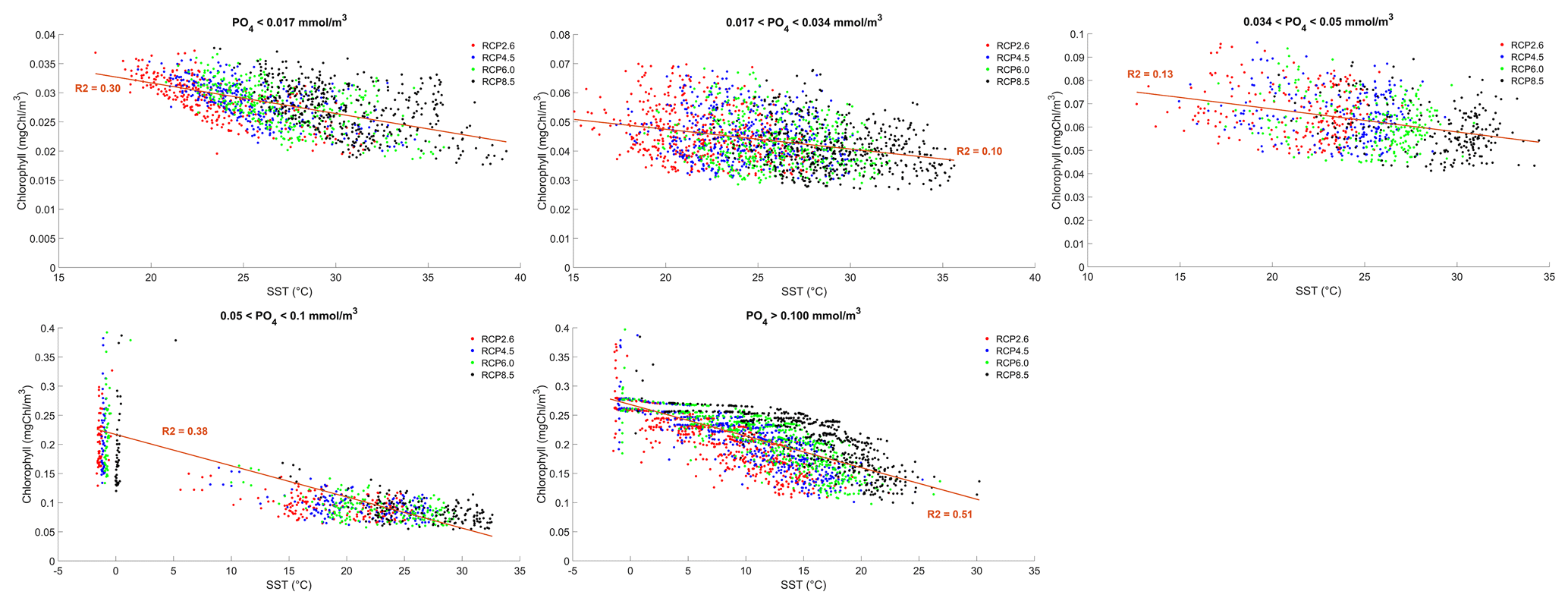
Figure A1Effect of SST (°C) on surface chlorophyll (mg Chl m−3) for each grid cell in the year 2500. The data are divided into five panels defined by their phosphate (PO4) concentrations. Red dots correspond to the simulations following the RCP2.6 scenario. Blue dots represent the simulations following the RCP4.5 scenario. Green dots represent the simulations following the RCP6.0 scenario. Black dots represent the simulations following the RCP8.5 scenario. The R2 value represents the coefficient of determination of the linear regression model
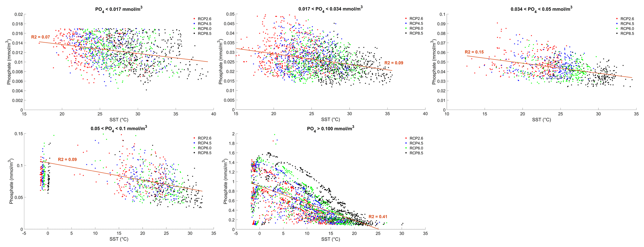
Figure A2Effect of SST (°C) on surface phosphate (PO4) concentrations (mmol m−3) for each grid cell in the year 2500. The data are divided into five panels defined by their PO4 concentrations. Red dots correspond to the simulations following the RCP2.6 scenario. Blue dots represent the simulations following the RCP4.5 scenario. Green dots represent the simulations following the RCP6.0 scenario. Black dots represent the simulations following the RCP8.5 scenario. The R2 value represents the coefficient of determination of the linear regression model
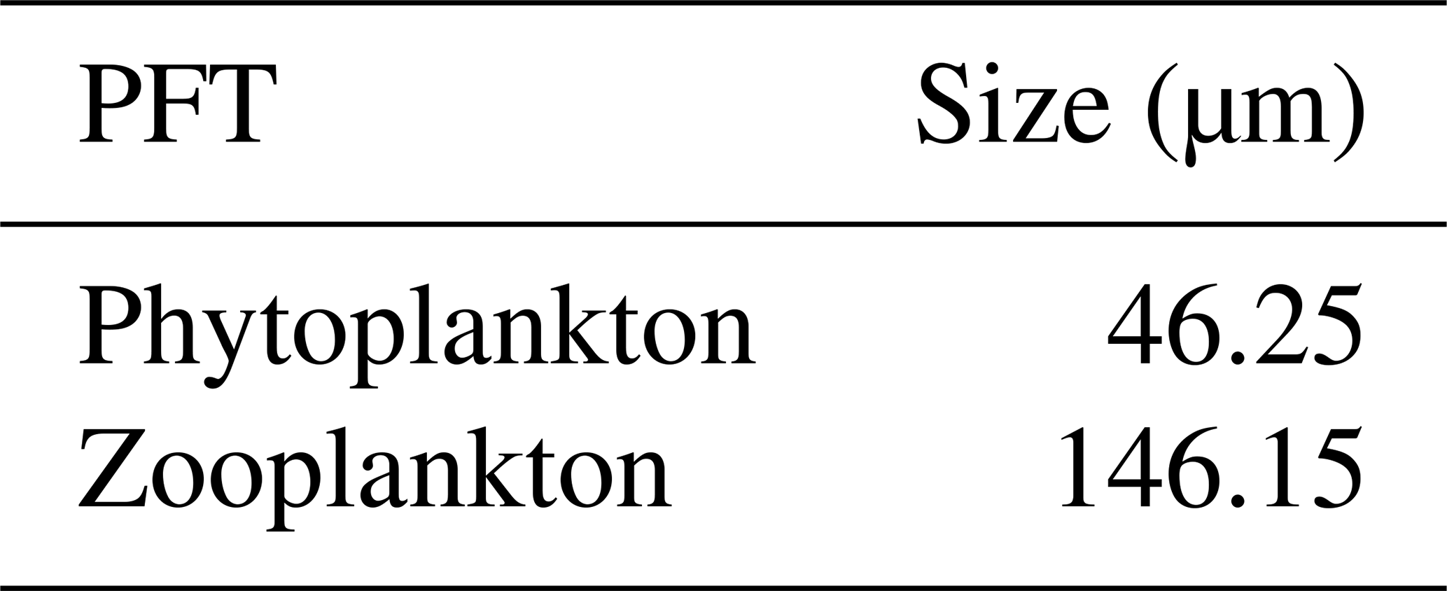
We base our ecosystem community on the one described by Ward et al. (2018). We only use 2 PFTs: one phytoplankton group and one zooplankton group (Table B1). We show that the complexity of the ecosystem does not have an important impact on the climate system compared to the effect of phytoplankton light absorption (Asselot et al., 2021). Therefore, for simplification, we reduce the ecosystem's complexity.
Table B1Size of the different plankton functional types (µm) used during the simulations.
To investigate how the ocean absorbs heat with and without phytoplankton light absorption, we computed the ocean heat content over the top 2000 m and between 60° N–60° S. Independently of the scenario, phytoplankton light absorption increases the ocean heat content in the top 2000 m. However, this increase strongly varies between scenarios. For instance, ocean heat content increases by 79 % for RCP2.6, while it only increases by 0.05 % for RCP8.5.
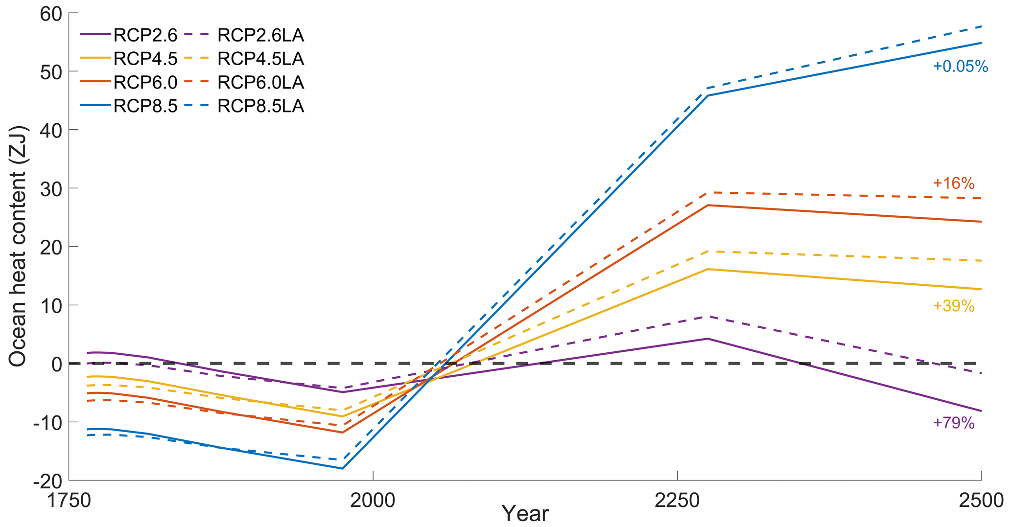
Figure C1Variations in ocean heat content (ZJ) in the top 2000 m between 60° N–60° S. The purple curves represent RCP2.6. The yellow curves represent RCP4.5. The orange curves represent RCP6.0. The blue curves represent RCP8.5. The dotted curves represent the simulations with phytoplankton light absorption, while the plain curves represent simulations without. The anomalies have been computed with respect to the mean of the time series.
Independent of the RCP scenarios, our results evidence an increase in surface nutrients, such as phosphate. As a result, the surface chlorophyll biomass increases with phytoplankton light absorption.
Table D1Changes in global oceanic CO2 concentration and air–sea CO2 flux between the simulations. The “−” symbol in the second column indicates a decrease in global oceanic CO2 concentration in the simulation with phytoplankton light absorption compared to the one without. The “+” symbol in the third column indicates an increase in air–sea CO2 flux in the simulation with phytoplankton light absorption compared to the one without.
To investigate the substantially reduced ocean CO2 uptake with phytoplankton light absorption, we continue our simulations for another 1000 years with no further CO2 emissions. The difference in atmospheric CO2 concentrations between the simulations with and without phytoplankton light absorption decreases with time. This result evidences that large CO2 differences are driven by a transient effect of reduced CO2 uptake fluxes, consistent with reduced CO2 solubility under phytoplankton light absorption warming.
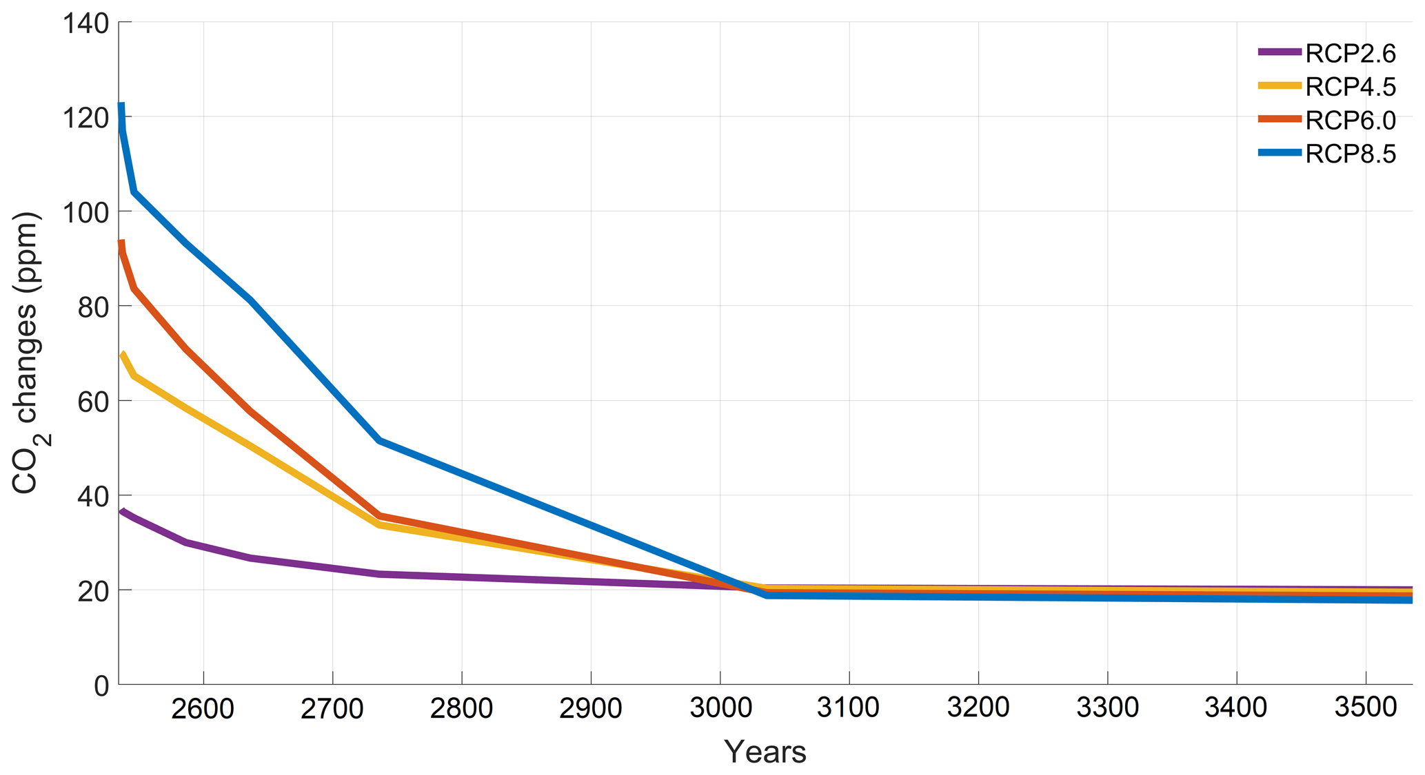
Figure E1Difference in atmospheric CO2 concentrations through time for the additional simulations.
Independent of the RCP scenarios, our results evidence an increase in surface nutrients, such as phosphate. As a result, the surface chlorophyll biomass increases with phytoplankton light absorption.
Table F1Phosphate concentration changes at the surface (mol kg−1) for the different RCP scenarios in the year 2500. The values represent the difference with minus without phytoplankton light absorption. The “+” symbol indicates an increase in surface PO4 concentration.

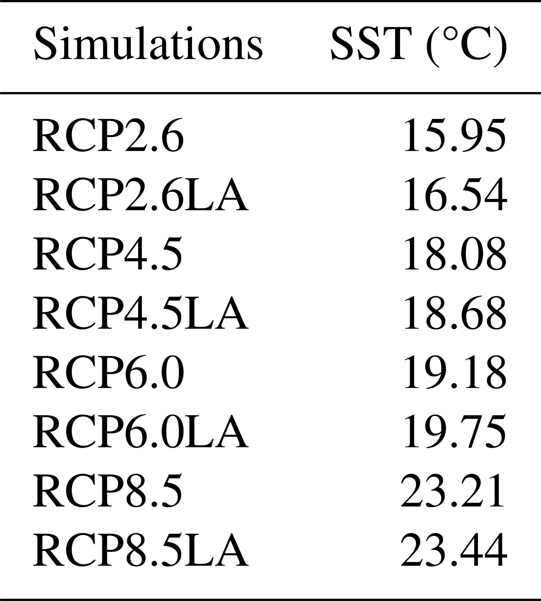
Table G1Sea surface temperature (°C) for the different simulations.
The code for the model is hosted on GitHub and can be obtained by cloning or downloading: https://doi.org/10.5281/zenodo.5676165 (Ridgwell et al., 2021). The configuration file is named “RA.ECO.ra32lv.FeTDTL.36x36x32” and can be found under the directory “EcoGENIE_LA/genie-main/configs”. The user configuration files to run the experiments can be found under the directory “EcoGENIE_LA/genie-userconfigs/RA/Asselotetal_ESD”. Details of the code installation and basic model configuration can be found in a PDF file (https://www.seao2.info/cgenie/docs/muffin.pdf, last access: 12 March 2021). Finally, Sect. 9 of the manual provides tutorials on the ECOGEM ecosystem model.
The greenhouse gas time series used in this study can be downloaded here: https://www.pik-potsdam.de/~mmalte/rcps/. A complete description of these time series is available in Meinshausen et al. (2011).
All authors designed and developed the concept of the study. RA performed the analysis of the model outputs with inputs from IH. RA drafted the initial version of the paper in collaboration with IH. All co-authors read and reviewed the final version of the paper.
The contact author has declared that none of the authors has any competing interests.
Publisher’s note: Copernicus Publications remains neutral with regard to jurisdictional claims made in the text, published maps, institutional affiliations, or any other geographical representation in this paper. While Copernicus Publications makes every effort to include appropriate place names, the final responsibility lies with the authors.
We thank the two anonymous reviewers and Sarah Berthet for their comments that improved the quality of the manuscript. Our special thanks go to Jana Hinners, Isabell Hochfeld, Félix Pellerin, Maike Scheffold and Laurin Steidle for their valuable comments on an earlier version of this manuscript.
This work was supported by the Center for Earth System Research and Sustainability (CEN), University of Hamburg, and contributes to the Cluster of Excellence “CLICCS – Climate, Climatic Change, and Society”.
This paper was edited by Roberta D'Agostino and reviewed by Sarah Berthet and two anonymous referees.
Anderson, S., Barton, A., Clayton, S., Dutkiewicz, S., and Rynearson, T.: Marine phytoplankton functional types exhibit diverse responses to thermal change, Nat. Commun., 12, 1–9, 2021. a
Anderson, W., Gnanadesikan, A., Hallberg, R., Dunne, J., and Samuels, B.: Impact of ocean color on the maintenance of the Pacific Cold Tongue, Geophys. Res. Lett., 34, L11609, https://doi.org/10.1029/2007GL030100, 2007. a
Asselot, R., Lunkeit, F., Holden, P. B., and Hense, I.: The relative importance of phytoplankton light absorption and ecosystem complexity in an Earth system model, J. Adv. Model. Earth Sy., 13, e2020MS002110, https://doi.org/10.1029/2020MS002110, 2021. a, b, c, d, e, f, g, h, i, j, k, l, m, n, o, p, q, r, s, t
Asselot, R., Lunkeit, F., Holden, P. B., and Hense, I.: Climate pathways behind phytoplankton-induced atmospheric warming, Biogeosciences, 19, 223–239, https://doi.org/10.5194/bg-19-223-2022, 2022. a, b, c, d, e
Behrenfeld, M. J. and Falkowski, P. G.: Photosynthetic rates derived from satellite–based chlorophyll concentration, Limnol. Oceanogr., 42, 1–20, 1997. a
Boyce, D. G., Dowd, M., Lewis, M. R., and Worm, B.: Estimating global chlorophyll changes over the past century, Prog. Oceanogr., 122, 163–173, 2014. a
Cael, B., Bisson, K., Boss, E., Dutkiewicz, S., and Henson, S.: Global climate-change trends detected in indicators of ocean ecology, Nature, 1–4, 2023. a
Cameron, D. R., Lenton, T. M., Ridgwell, A. J., Shepherd, J. G., Marsh, R., and Yool, A.: A factorial analysis of the marine carbon cycle and ocean circulation controls on atmospheric CO2, Global Biogeochem. Cy., 19, GB4027, https://doi.org/10.1029/2005GB002489, 2005. a
Capone, D. G., Subramaniam, A., Montoya, J. P., Voss, M., Humborg, C., Johansen, A. M., Siefert, R. L., and Carpenter, E. J.: An extensive bloom of the N2-fixing cyanobacterium Trichodesmium erythraeum in the central Arabian Sea, Mar. Ecol.-Prog. Ser., 172, 281–292, 1998. a
Claussen, M., Mysak, L., Weaver, A., Crucifix, M., Fichefet, T., Loutre, M.-F., Weber, S., Alcamo, J., Alexeev, V., Berger, A., Calov, R., Ganopolski, A., Goosse, H., Lohmann, G., Lunkeit, F., Mokhov, I., Petoukhov, V., Stone, P., and Wang, W.: Earth system models of intermediate complexity: closing the gap in the spectrum of climate system models, Clim. Dynam., 18, 579–586, 2002. a
Conkright, M. E.: World Ocean Atlas 2001. Volume 4, Nutrients, edited by: Levitus, S., NOAA Atlas NESDIS, 1102, 2002. a
Edwards, N. R. and Marsh, R.: Uncertainties due to transport-parameter sensitivity in an efficient 3-D ocean-climate model, Clim. Dynam., 24, 415–433, 2005. a, b
Geider, R. J., Maclntyre, H. L., and Kana, T. M.: A dynamic regulatory model of phytoplanktonic acclimation to light, nutrients, and temperature, Limnol. Oceanogr., 43, 679–694, 1998. a, b
Gibbs, S. J., Bown, P. R., Ridgwell, A., Young, J. R., Poulton, A. J., and O'Dea, S. A.: Ocean warming, not acidification, controlled coccolithophore response during past greenhouse climate change, Geology, 44, 59–62, 2016. a
Goldman, J. C.: Temperature effects on phytoplankton growth in continuous culture, Limnol. Oceanogr., 22, 932–936, 1977. a
Greene, S., Ridgwell, A., Kirtland Turner, S., Schmidt, D. N., Pälike, H., Thomas, E., Greene, L., and Hoogakker, B.: Early Cenozoic decoupling of climate and carbonate compensation depth trends, Paleoceanogr. Paleocl., 34, 930–945, 2019. a
Hense, I.: Regulative feedback mechanisms in cyanobacteria-driven systems: a model study, Mar. Ecol.-Prog. Ser., 339, 41–47, 2007. a
Henson, S. A., Sarmiento, J. L., Dunne, J. P., Bopp, L., Lima, I., Doney, S. C., John, J., and Beaulieu, C.: Detection of anthropogenic climate change in satellite records of ocean chlorophyll and productivity, Biogeosciences, 7, 621–640, https://doi.org/10.5194/bg-7-621-2010, 2010. a
Hibler, W. D.: A dynamic thermodynamic sea ice model, J. Phys. Oceanogr., 9, 815–846, 1979. a
Holden, P. B., Edwards, N. R., Müller, S. A., Oliver, K. I. C., Death, R. M., and Ridgwell, A.: Controls on the spatial distribution of oceanic δ13CDIC, Biogeosciences, 10, 1815–1833, https://doi.org/10.5194/bg-10-1815-2013, 2013. a
Holden, P. B., Edwards, N. R., Fraedrich, K., Kirk, E., Lunkeit, F., and Zhu, X.: PLASIM–GENIE v1.0: a new intermediate complexity AOGCM, Geosci. Model Dev., 9, 3347–3361, https://doi.org/10.5194/gmd-9-3347-2016, 2016. a
Kahru, M., Leppanen, J.-M., and Rud, O.: Cyanobacterial blooms cause heating of the sea surface, Mar. Ecol.-Prog. Ser., 101, 1–7, 1993. a
Kvale, K. F. and Meissner, K. J.: Primary production sensitivity to phytoplankton light attenuation parameter increases with transient forcing, Biogeosciences, 14, 4767–4780, https://doi.org/10.5194/bg-14-4767-2017, 2017. a, b
Kwiatkowski, L., Torres, O., Bopp, L., Aumont, O., Chamberlain, M., Christian, J. R., Dunne, J. P., Gehlen, M., Ilyina, T., John, J. G., Lenton, A., Li, H., Lovenduski, N. S., Orr, J. C., Palmieri, J., Santana-Falcón, Y., Schwinger, J., Séférian, R., Stock, C. A., Tagliabue, A., Takano, Y., Tjiputra, J., Toyama, K., Tsujino, H., Watanabe, M., Yamamoto, A., Yool, A., and Ziehn, T.: Twenty-first century ocean warming, acidification, deoxygenation, and upper-ocean nutrient and primary production decline from CMIP6 model projections, Biogeosciences, 17, 3439–3470, https://doi.org/10.5194/bg-17-3439-2020, 2020. a
Laufkötter, C., Vogt, M., Gruber, N., Aita-Noguchi, M., Aumont, O., Bopp, L., Buitenhuis, E., Doney, S. C., Dunne, J., Hashioka, T., Hauck, J., Hirata, T., John, J., Le Quéré, C., Lima, I. D., Nakano, H., Seferian, R., Totterdell, I., Vichi, M., and Völker, C.: Drivers and uncertainties of future global marine primary production in marine ecosystem models, Biogeosciences, 12, 6955–6984, https://doi.org/10.5194/bg-12-6955-2015, 2015. a, b
Lewis, M. R., Cullen, J. J., and Platt, T.: Phytoplankton and thermal structure in the upper ocean: consequences of nonuniformity in chlorophyll profile, J. Geophys. Res.-Oceans, 88, 2565–2570, 1983. a
Mahowald, N. M., Yoshioka, M., Collins, W. D., Conley, A. J., Fillmore, D. W., and Coleman, D. B.: Climate response and radiative forcing from mineral aerosols during the last glacial maximum, pre-industrial, current and doubled-carbon dioxide climates, Geophys. Res. Lett., 33, L20705, https://doi.org/10.1029/2006GL026126, 2006. a
Manizza, M., Le Quéré, C., Watson, A. J., and Buitenhuis, E. T.: Bio-optical feedbacks among phytoplankton, upper ocean physics and sea-ice in a global model, Geophys. Res. Lett., 32, L05603, https://doi.org/10.1029/2004GL020778, 2005. a, b
McClain, C. R., Signorini, S. R., and Christian, J. R.: Subtropical gyre variability observed by ocean-color satellites, Deep-Sea Res. Pt. II, 51, 281–301, 2004. a
Meinshausen, M., Smith, S. J., Calvin, K., Daniel, J. S., Kainuma, M. L. T., Lamarque, J.-F., Matsumoto, K., Montzka, S.A., Raper, S. C. B., Riahi, K., Thomson, A., Velders, G. J. M., and van Vuuren, D. P. P.: The RCP greenhouse gas concentrations and their extensions from 1765 to 2300, Climatic Change, 109, 213, https://doi.org/10.1007/s10584-011-0156-z, 2011 (data available at: https://www.pik-potsdam.de/~mmalte/rcps/, last access: 10 July 2024). a, b, c, d
Meyer, K., Ridgwell, A., and Payne, J.: The influence of the biological pump on ocean chemistry: implications for long-term trends in marine redox chemistry, the global carbon cycle, and marine animal ecosystems, Geobiology, 14, 207–219, 2016. a
Moore, J. K., Doney, S. C., Kleypas, J. A., Glover, D. M., and Fung, I. Y.: An intermediate complexity marine ecosystem model for the global domain, Deep-Sea Res. Pt. II, 49, 403–462, 2001. a
Moss, R. H., Edmonds, J. A., Hibbard, K. A., Manning, M. R., Rose, S. K., Van Vuuren, D. P., Carter, T. R., Emori, S., Kainuma, M., Kram, T., Meehl, G. A., Mitchell, J. F. B., Nakicenovic, N., Riahi, K., Smith, S. J., Stouffer, R. J., Thomson, A. M., Weyant, J. P., and Wilbanks, T. J.: The next generation of scenarios for climate change research and assessment, Nature, 463, 747–756, 2010. a, b
Park, J.-Y., Kug, J.-S., Bader, J., Rolph, R., and Kwon, M.: Amplified Arctic warming by phytoplankton under greenhouse warming, P. Natl. Acad. Sci. USA, 112, 5921–5926, 2015. a, b
Patara, L., Vichi, M., Masina, S., Fogli, P. G., and Manzini, E.: Global response to solar radiation absorbed by phytoplankton in a coupled climate model, Clim. Dynam., 39, 1951–1968, 2012. a, b, c, d, e, f, g, h
Paulsen, H.: The effects of marine nitrogen-fixing cyanobacteria on ocean biogeochemistry and climate – an Earth system model perspective, PhD thesis, Universität Hamburg Hamburg, https://doi.org/10.17617/2.2598976, 2018. a, b, c
Pellerin, F., Porada, P., and Hense, I.: ESD Reviews: Evidence of multiple inconsistencies between representations of terrestrial and marine ecosystems in Earth System Models, Earth Syst. Dynam. Discuss. [preprint], https://doi.org/10.5194/esd-2020-55, 2020. a, b
Polovina, J. J., Howell, E. A., and Abecassis, M.: Ocean's least productive waters are expanding, Geophys. Res. Lett., 35, L03618, https://doi.org/10.1029/2007GL031745, 2008. a
Reale, M., Cossarini, G., Lazzari, P., Lovato, T., Bolzon, G., Masina, S., Solidoro, C., and Salon, S.: Acidification, deoxygenation, and nutrient and biomass declines in a warming Mediterranean Sea, Biogeosciences, 19, 4035–4065, https://doi.org/10.5194/bg-19-4035-2022, 2022. a
Reinhard, C. T., Planavsky, N. J., Ward, B. A., Love, G. D., Le Hir, G., and Ridgwell, A.: The impact of marine nutrient abundance on early eukaryotic ecosystems, Geobiology, 18, 139–151, 2020. a
Rhee, G.-Y. and Gotham, I. J.: The effect of environmental factors on phytoplankton growth: temperature and the interactions of temperature with nutrient limitation, Limnol. Oceanogr., 26, 635–648, 1981. a
Richon, C., Dutay, J.-C., Bopp, L., Le Vu, B., Orr, J. C., Somot, S., and Dulac, F.: Biogeochemical response of the Mediterranean Sea to the transient SRES-A2 climate change scenario, Biogeosciences, 16, 135–165, https://doi.org/10.5194/bg-16-135-2019, 2019. a
Ridgwell, A., Hargreaves, J. C., Edwards, N. R., Annan, J. D., Lenton, T. M., Marsh, R., Yool, A., and Watson, A.: Marine geochemical data assimilation in an efficient Earth System Model of global biogeochemical cycling, Biogeosciences, 4, 87–104, https://doi.org/10.5194/bg-4-87-2007, 2007. a, b, c, d, e
Ridgwell, A., Reinhard, C., van de Velde, S., Asselot, R., Adloff, M., Wilson, J., Ward, B., Hülse, D., Monteiro, F., and Vervoort, P.: crem33/EcoGENIE_LA: Asselotetal2021_ESD (Asselotetal2021_ESD), Zenodo [code], https://doi.org/10.5281/zenodo.5676165, 2021. a
Schlunegger, S., Rodgers, K. B., Sarmiento, J. L., Ilyina, T., Dunne, J. P., Takano, Y., Christian, J. R., Long, M. C., Frölicher, T. L., Slater, R., and Lehner, F.: Time of emergence and large ensemble intercomparison for ocean biogeochemical trends, Global Biogeochem. Cy., 34, e2019GB006453, https://doi.org/10.1029/2019GB006453, 2020. a
Semtner, A. J.: A model for the thermodynamic growth of sea ice in numerical investigations of climate, J. Phys. Oceanogr., 6, 379–389, 1976. a
Shell, K., Frouin, R., Nakamoto, S., and Somerville, R.: Atmospheric response to solar radiation absorbed by phytoplankton, J. Geophys. Res.-Atmos., 108, 4445, https://doi.org/10.1029/2003JD003440, 2003. a, b, c
Sonntag, S.: Modeling biological-physical feedback mechanisms in marine systems, PhD thesis, Universität Hamburg, Hamburg, https://ediss.sub.uni-hamburg.de/handle/ediss/5134 (last access: 9 July 2024), 2013. a, b, c, d
Stockey, R. G., Pohl, A., Ridgwell, A., Finnegan, S., and Sperling, E. A.: Decreasing Phanerozoic extinction intensity as a consequence of Earth surface oxygenation and metazoan ecophysiology, P. Natl. Acad. Sci. USA, 118, e2101900118, https://doi.org/10.1073/pnas.2101900118, 2021. a
Tagliabue, A., Kwiatkowski, L., Bopp, L., Butenschön, M., Cheung, W., Lengaigne, M., and Vialard, J.: Persistent Uncertainties in Ocean Net Primary Production Climate Change Projections at Regional Scales Raise Challenges for Assessing Impacts on Ecosystem Services, Frontiers in Climate, 3, 738224, https://doi.org/10.3389/fclim.2021.738224, 2021. a
Thompson, S. L. and Warren, S. G.: Parameterization of outgoing infrared radiation derived from detailed radiative calculations, J. Atmos. Sci., 39, 2667–2680, 1982. a
Trenberth, K. E.: A global ocean wind stress climatology based on ECMWF analyses, NCAR Tech. note, 93, https://cir.nii.ac.jp/crid/1572543024240012928 (last access: 9 July 2024), 1989. a
Wanninkhof, R.: Relationship between wind speed and gas exchange over the ocean, J. Geophys. Res.-Oceans, 97, 7373–7382, 1992. a
Ward, B. A., Wilson, J. D., Death, R. M., Monteiro, F. M., Yool, A., and Ridgwell, A.: EcoGEnIE 1.0: plankton ecology in the cGEnIE Earth system model, Geosci. Model Dev., 11, 4241–4267, https://doi.org/10.5194/gmd-11-4241-2018, 2018. a, b, c, d, e, f, g, h, i, j, k, l
Weaver, A. J., Eby, M., Wiebe, E. C., Bitz, C. M., Duffy, P. B., Ewen, T. L., Fanning, A. F., Holland, M. M., MacFadyen, A., Matthews, H. D., Meissner, K. J., Saenko, O., Schmittner, A., Wang, H., and Yoshimori, M.: The UVic Earth System Climate Model: Model description, climatology, and applications to past, present and future climates, Atmos.-Ocean, 39, 361–428, 2001. a, b
Wetzel, P., Maier-Reimer, E., Botzet, M., Jungclaus, J., Keenlyside, N., and Latif, M.: Effects of ocean biology on the penetrative radiation in a coupled climate model, J. Climate, 19, 3973–3987, 2006. a, b
Wilson, J., Monteiro, F., Schmidt, D., Ward, B., and Ridgwell, A.: Linking marine plankton ecosystems and climate: A new modeling approach to the warm early Eocene climate, Paleoceanogr. Paleocl., 33, 1439–1452, 2018. a
Wurl, O., Bird, K., Cunliffe, M., Landing, W. M., Miller, U., Mustaffa, N. I. H., Ribas-Ribas, M., Witte, C., and Zappa, C. J.: Warming and inhibition of salinization at the ocean's surface by cyanobacteria, Geophys. Res. Lett., 45, 4230–4237, 2018. a
Zickfeld, K., Eby, M., Weaver, A. J., Alexander, K., Crespin, E., Edwards, N. R., Eliseev, A. V., Feulner, G., Fichefet, T., Forest, C. E., Friedlingstein, P., Goosse, H., Holden, P. B., Joos, F., Kawamiya, M., Kicklighter, D., Kienert, H., Matsumoto, K., Mokhov, I. I., Monier, E., Olsen, S. M., Pedersen, J. O. P., Perrette, M., Philippon-Berthier, G., Ridgwell, A., Schlosser, A., Schneider Von Deimling, T., Shaffer, G., Sokolov, A., Spahni, R., Steinacher, M., Tachiiri, K., Tokos, K. S., Yoshimori, M., Zeng, N., and Zhao, F.: Long-term climate change commitment and reversibility: an EMIC intercomparison, J. Climate, 26, 5782–5809, 2013. a, b, c, d, e, f
- Abstract
- Introduction
- Methods
- Results
- Discussion and conclusions
- Appendix A: Optimum net phytoplankton growth
- Appendix B: Plankton functional types
- Appendix C: Ocean heat content
- Appendix D: Carbon dioxide
- Appendix E: Additional simulations
- Appendix F: Surface phosphate concentration
- Appendix G: Sea surface temperature
- Code availability
- Data availability
- Author contributions
- Competing interests
- Disclaimer
- Acknowledgements
- Financial support
- Review statement
- References