the Creative Commons Attribution 4.0 License.
the Creative Commons Attribution 4.0 License.
 | 08 Aug 2024
Similar North Pacific variability despite suppressed El Niño variability in the warm mid-Pliocene climate
Michiel L. J. Baatsen
Anna S. von der Heydt
Frank M. Selten
Henk A. Dijkstra
The mid-Pliocene is the most recent geological period with similar atmospheric CO2 concentration to the present day and similar surface temperatures to those projected at the end of this century for a moderate warming scenario. While not a perfect analogue, the mid-Pliocene can be used to study the functioning of the Earth system under similar forcings to a near future, especially regarding features in the climate system for which uncertainties exist in future projections. According to the Pliocene Model Intercomparison Project Phase 2 (PlioMIP2), the variability in the El Niño–Southern Oscillation (ENSO) was suppressed. In this study, we investigate how teleconnections of ENSO, specifically variability in the North Pacific atmosphere, respond to a suppressed ENSO according to PlioMIP2. The multi-model mean (MMM) shows a similar sea-level pressure (SLP) variability in the Aleutian Low (AL) in the mid-Pliocene and pre-industrial, but a per-model view reveals that the change in AL variability is related to the change in ENSO variability. Even though ENSO is suppressed, the teleconnection between ENSO sea-surface temperature (SST) anomalies, tropical precipitation, and North Pacific SLP anomalies is quite robust in the mid-Pliocene. We split AL variability in a part that is ENSO-related, and a residual variability which is related to internal stochastic variability, and find that the change in ENSO-related AL variability is strongly related to the change in ENSO variability itself, while the change in residual AL variability is unrelated to ENSO change. Since the internal atmospheric variability, which is the dominant forcing of the AL variability, is largely unchanged, we are able to understand that the AL variability is largely similar even though ENSO variability is suppressed. We find that the specific change in ENSO and AL variability depends on both the model equilibrium climate sensitivity and Earth system sensitivity. Finally, we present a perspective of (extra-)tropical Pacific variability in PlioMIP2, combining our results with literature findings on changes in the tropical mean climate and in the Pacific Decadal Oscillation (PDO).
- Article
(3076 KB) - Full-text XML
-
Supplement
(3755 KB) - BibTeX
- EndNote


The mid-Pliocene (∼3 Ma) is the most recent geological period that had a similar atmospheric CO2 concentration to the present day (∼400 ppm; de la Vega et al., 2020). Its global surface temperatures were similar to those projected for the end of this century following the SSP2-4.5 future climate scenario (Tierney et al., 2020). Apart from elevated atmospheric CO2, the mid-Pliocene had a similar geography – compared to earlier geological warm periods – to the present day (Haywood et al., 2011). Notable differences include a reduction in the Greenland and West Antarctic ice sheets; closure of the Bering Strait and Canadian Arctic Archipelago; and changes to topography, bathymetry, and vegetation (Dowsett et al., 2016). Because of these similarities, the mid-Pliocene climate has been called the “best analogue” to near-future climate in comparison to other past warm periods (Burke et al., 2018). Regardless of its potential as a future climate analogue, the mid-Pliocene can serve as a benchmark for climate models. The analysis of the climate system under mid-Pliocene boundary conditions can help us investigate the strength of feedbacks and the response of large-scale climate features to specific forcings.
The first coordinated effort to simulate the mid-Pliocene climate was the first phase of the Pliocene Model Intercomparison Project (PlioMIP; Haywood et al., 2010). It was followed by PlioMIP2 (Haywood et al., 2016), and the most recent phase, PlioMIP3, has just been announced (Haywood et al., 2024). PlioMIP2 was specifically designed to reduce model–proxy uncertainties. All models are supplied with consistent boundary conditions, which are focused on a specific time slice (KM5c interglacial, 3.205 Ma) where the orbital configuration was close to present-day conditions (Haywood et al., 2016; Dowsett et al., 2016).
In the past years, many studies of the mid-Pliocene climate based on PlioMIP2 have been published. In the global mean, the mid-Pliocene climate was 3.3 °C warmer than the pre-industrial climate (ranging between +1.7 and +5.2 °C) (Haywood et al., 2020). Increased CO2 and closed gateways influenced the Arctic such that Arctic temperatures were relatively high due to Arctic amplification (De Nooijer et al., 2020). Most models simulate summer Arctic sea-ice-free conditions, and the Atlantic Meridional Overturning Circulation (AMOC) was intensified (De Nooijer et al., 2020; Weiffenbach et al., 2023). Atmospheric moisture content was increased, leading to more precipitation on average (Haywood et al., 2020) and specifically wetter conditions over the deep tropics, such as the Pacific Intertropical Convergence Zone (ITCZ, Han et al., 2021). The subtropics become drier over the ocean, but precipitation over land is generally enhanced related to enhanced monsoonal activity (Berntell et al., 2021; Feng et al., 2022). A hemispheric energy asymmetry shifts the Hadley circulation and ITCZ northwards (Han et al., 2021; Zhang et al., 2024). The Pacific Walker circulation is shifted westward (Han et al., 2021; Zhang et al., 2024), and this is associated with warmer and wetter conditions over the Indian Ocean and the Maritime Continent (Ren et al., 2023). Not all of these features are analogous to (near-)future climate projections; e.g. AMOC is projected to decrease, while the mid-Pliocene AMOC is simulated to be strengthened (Eyring et al., 2021; Weiffenbach et al., 2023).
A more puzzling feature of the mid-Pliocene climate is the behaviour of the El Niño–Southern Oscillation (ENSO). In the present day, ENSO is the dominant mode of climate variability on interannual timescales, with teleconnections to many regions of the world (Philander, 1990). Earlier work using proxy reconstructions showed a reduced zonal sea-surface temperature (SST) gradient in the tropical Pacific mean climate (Wara et al., 2005; Ravelo et al., 2006), on the basis of which it was suggested that the mid-Pliocene ENSO was settled in a “permanent El Niño” state (Fedorov et al., 2006). Proxies for variability in the mid-Pliocene do suggest, however, that there existed ENSO variability with an amplitude varying between reduced and similar to the present day (Scroxton et al., 2011; Watanabe et al., 2011; White and Ravelo, 2020). In addition, more recent reconstructions and modelling efforts suggest that the zonal SST gradient is not as reduced as previously thought and that it could be in line with model estimates (Zhang et al., 2014; Tierney et al., 2019). Modelling efforts in PlioMIP1 (Brierley, 2015) and PlioMIP2 (Oldeman et al., 2021) agree with that finding, showing that ENSO variability was reduced in the majority of the models but with considerable spread in the model ensemble. The suppression of ENSO in PlioMIP2 is explained by a series of off-equatorial processes triggered by the northward displacement of the Pacific ITCZ (Pontes et al., 2022).
ENSO variability exerts a global influence through its oceanic and atmospheric teleconnections, which include a circumglobal connection along the tropics and links with the stratosphere (Yeh et al., 2018; Cai et al., 2019; Domeisen et al., 2019). The so-called “atmospheric bridge” explains the deterministic link between ENSO and the variability in the North Pacific atmosphere and ocean, in which SST anomalies originating from ENSO events cause extratropical atmospheric variability via tropical convection, the Hadley circulation, and atmospheric Rossby waves (Hoskins and Karoly, 1981; Mo and Livezey, 1986; Alexander et al., 2002). The variability in the North Pacific atmosphere is often referred to as Aleutian Low (AL) variability, which consists of the dominant Pacific–North American (PNA) pattern and the second-leading North Pacific Oscillation (NPO) (Barnston and Livezey, 1987; Linkin and Nigam, 2008). AL variability is in part forced by ENSO through the deterministic atmospheric bridge but also by internal stochastic variability (Di Lorenzo et al., 2013; Newman et al., 2016). The dominant mode of ocean variability in the North Pacific is the Pacific Decadal Oscillation (PDO), which is forced by AL variability through wind forcing and by ENSO through ocean waves (Newman et al., 2003, 2016; Di Lorenzo and Mantua, 2016).
What may happen to ENSO and its teleconnections to the North Pacific in the near future under global warming is unclear. It is likely that ENSO–precipitation variability will increase (Cai et al., 2021; Yun et al., 2021) and that the variability in ENSO and atmospheric teleconnections, including AL variability, will increase in the near future (Chen et al., 2018; Fredriksen et al., 2020; Cai et al., 2021). However, uncertainties are very large, in part due to internal variability, and conclusions become even less robust towards the end of this century (Fredriksen et al., 2020; Beobide-Arsuaga et al., 2021). Additionally, ENSO teleconnections can also change because mean atmospheric circulation will change, regardless of ENSO change (Yeh et al., 2018). In the long term, idealized future warming simulations under equilibrated high CO2 forcing, however, suggest a weakening of ENSO variability (Callahan et al., 2021; Zheng et al., 2022). This is similar to what is found in PlioMIP2 (Oldeman et al., 2021; Pontes et al., 2022), implying that the mid-Pliocene ENSO response is similar to what could be expected in an equilibrated high-CO2 future but is not similar to the near-future ENSO response. This makes the mid-Pliocene climate a valuable test case to investigate the response of North Pacific variability to a suppressed ENSO.
Although ENSO variability is reduced compared to the pre-industrial in the majority of PlioMIP2 models (Oldeman et al., 2021), the amplitude of the PDO variability does not change, at least in a subset of the PlioMIP2 ensemble, making the PDO the dominant mode of ocean variability in the Pacific sector (Katya Canal-Solis, personal communications, 2024). However, there is a considerable model spread regarding both ENSO and PDO change in PlioMIP2. In one PlioMIP2 model, it is the mid-Pliocene boundary conditions that cause an ENSO suppression and substantial suppression of the AL variability (specifically the PNA pattern), while elevated CO2 causes increased AL variability without any change in ENSO (Oldeman et al., 2023). It could indicate a tug of war in ENSO teleconnection responses to different conditions of the mid-Pliocene. However, the model used in Oldeman et al. (2023) showed the largest ENSO reduction of PlioMIP2, so it might not be representative of the rest of the ensemble.
In this study, we aim to answer the following question: how does variability in the North Pacific atmosphere respond to a suppressed ENSO in the warm mid-Pliocene climate, according to the PlioMIP2 ensemble? Specifically, we want to know the following. (1) Is any change in AL variability related to the change in ENSO? (2) Does the ENSO–North Pacific atmosphere teleconnection strength change? (3) Are there any changes in the North Pacific variability not related to ENSO change? And (4) is the ENSO teleconnection response related to model–climate sensitivity? To answer these questions, we will investigate simulation results of the PlioMIP2 ensemble. More details on the simulations and the analysis methods are presented in Sect. 2. Section 3 presents the results and provides answers to the research questions. In Sect. 4, we discuss the results and interpret our findings. We conclude with a summary in Sect. 5.
2.1 Models, simulations, and data
2.1.1 The PlioMIP2 ensemble
The PlioMIP2 ensemble consists of 17 climate models (Table 1). All models performed simulations following the PlioMIP2 protocol, which includes a pre-industrial control reference simulation (E280) and a mid-Pliocene simulation (Eoi400) (Haywood et al., 2016). Pre-industrial simulations are forced with 280 ppm atmospheric CO2, while the mid-Pliocene simulations are forced with 400 ppm CO2. Altered mid-Pliocene boundary conditions include closed Arctic gateways (Bering Strait and Canadian Arctic Archipelago); reduced land-ice cover (Greenland ice sheet and West Antarctic Ice Sheet); shoaling of the Sunda and Sahul shelves leading to changes to straits in the Maritime Continent; and changes to vegetation, lakes, and soils (Dowsett et al., 2016; Haywood et al., 2016). Only HadGEM3 used a modern land–sea mask in the Eoi400 simulation (Williams et al., 2021). All model simulations were run for 1000 or more model years (following PlioMIP2 protocol) and can be regarded as being in climatological equilibrium. We use the last 100 years from each simulation.
Feng et al. (2020)Chandan and Peltier (2017)Baatsen et al. (2022)Feng et al. (2020)Feng et al. (2020)Stepanek et al. (2020)Zheng et al. (2019)Hunter et al. (2019)Williams et al. (2021)Tan et al. (2020)Tan et al. (2020)Lurton et al. (2020)Chan and Abe-Ouchi (2020)Kamae et al. (2016)Li et al. (2020)Li et al. (2020)Table 1Details of the models contributing to the PlioMIP2 ensemble, with equilibrium climate sensitivity (ECS) and Earth system sensitivity (ESS) from Haywood et al. (2020) and Williams et al. (2021). In bold are the models primarily used in this study. The asterisks (*) show when the model has sensitivity simulations available (either E400 or Eoi280).
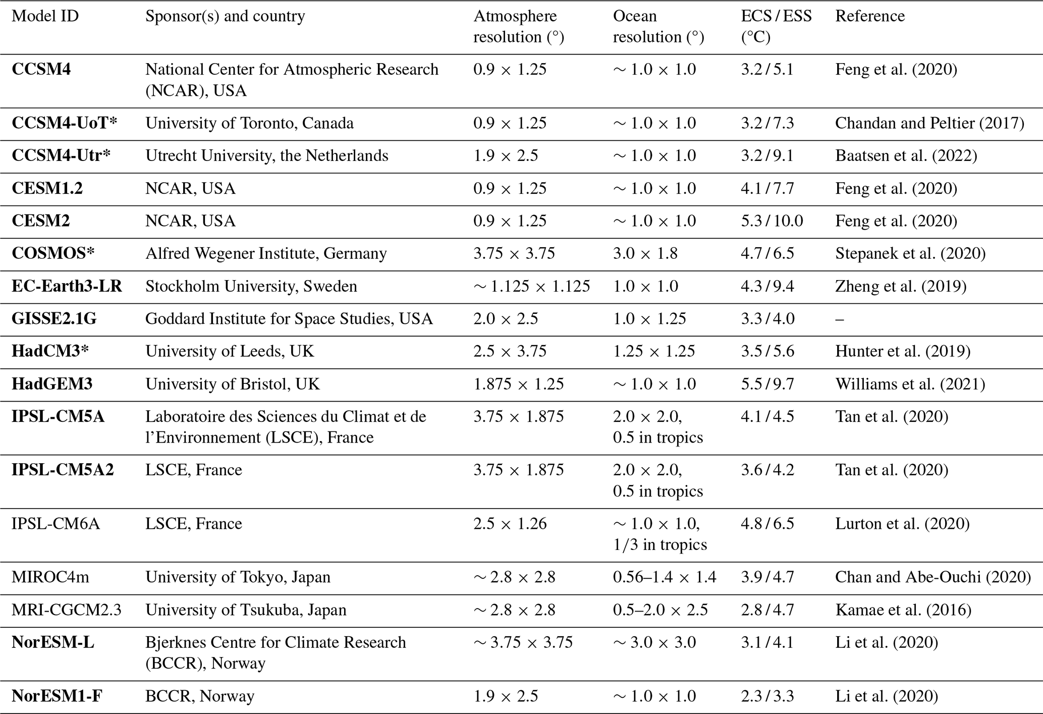
Additionally, we use two different sensitivity simulations that are available for a subset of PlioMIP2 models. We consider simulations with mid-Pliocene boundary conditions (BCs) but at pre-industrial CO2 levels (Eoi280), ran by CCSM4-Utr, COSMOS and HadCM3. We also consider simulations with mid-Pliocene CO2 levels but pre-industrial conditions otherwise (E400), ran by CCSM4-UoT, COSMOS and HadCM3.
2.1.2 Observational data
We compare the pre-industrial results to observational products of the present day and the historical period. For SSTs, we use the NOAA Extended Reconstructed SST (ERSST) v5 dataset (Huang et al., 2017). For atmospheric variables, we use the NOAA 20th Century Reanalysis (20CR) project v3 (Slivinski et al., 2021). We will refer to both products as “NOAA observations”. For consistency, we use 100 years, namely 1916–2015. These NOAA products have data available from the 19th century, which might be more like the pre-industrial, but the caveat is that the data become less reliable, so we chose to use recent data with higher reliability and consistency instead.
2.2 Analysis methods
We use 100 years of monthly SST, sea-level pressure (SLP), and total precipitation fields. For anomalies, we remove the climatology and a linear trend. For NOAA observations, we instead perform a LOWESS filtering (50-year running mean) to remove the trend from anthropogenic climate change. For model data, performing LOWESS filtering instead of removing a linear trend did not make any difference to the results. When computing multi-model means (MMMs) in space, we interpolate the model data on a rectilinear ∼1° grid.
We study variability through defined climate indices. We study ENSO variability through SST anomalies in the Niño 3.4 region (5° S–5° N, 150–90° W), which was also shown to capture ENSO variability well in the mid-Pliocene (Oldeman et al., 2021). To study Aleutian Low (AL) variability, we use SLP anomalies in the AL region (30–65° N, 160° E–140° W), also known as the North Pacific Index (Trenberth and Hurrell, 1994; Chen et al., 2020). This region also captures AL variability in the mid-Pliocene simulations, as shown in the Results section. We study precipitation variability in the western equatorial Pacific (WEP), which is the region that has the strongest ENSO-related precipitation anomalies (Deser and Wallace, 1990; Williams et al., 2024), defined here as 6° S–6° N, 120–180° E following Oldeman et al. (2023). In all cases we take area averages using grid weights based on the cosine of the latitude. Amplitudes of variability are generally defined as the standard deviation (SD) of the associated time series.
In order to connect ENSO teleconnections to other modes of variability, we compute the linear regression (linear slope) and correlation between the climate indices, where we quantify the teleconnection strength by means of the linear regression (e.g. Williams et al., 2024). Correlations are assumed statistically significant only if the corresponding p-value is below 0.05. Since the ENSO signal is strongest in boreal winter, we focus on the DJF mean Niño 3.4 index. The present-day ENSO leads AL variability, and we focus on the AL variability in DJFM. These months are chosen because the atmospheric response can take ∼1–2 weeks (e.g. Trenberth and Hurrell, 1994; Alexander et al., 2002; Newman et al., 2016). We test whether this assumption is valid by computing the lead–lag correlations between ENSO and the AL time series, and we find that ENSO leads AL with a 0–1 month lag with strongest correlations around January Niño 3.4 for NOAA observations and the majority of the models (Fig. S1 in the Supplement).
The deterministic teleconnection linking ENSO and AL variability, the atmospheric bridge, consists of several steps. ENSO SST anomalies leading to tropical convection anomalies (i.e. precipitation anomalies) are an important precursor to extratropical SLP anomalies in the North Pacific. Examining this step is relevant considering the substantial changes in the Indo-Pacific mean hydrological cycle in PlioMIP2 (e.g. Han et al., 2021; Ren et al., 2023; Zhang et al., 2024). Therefore, we also consider the regression between the Niño 3.4 index and tropical precipitation and the regression between WEP precipitation and North Pacific SLP anomalies.
Since we are interested in the ENSO–AL teleconnection change in the mid-Pliocene, we check whether the PlioMIP2 models are able to simulate that connection well in the pre-industrial. We find that IPSL-CM6A, MIROC4m, and MRI-CGCM2.3 do not show statistically significant correlations between the Niño 3.4 and AL indices in the E280 simulation in any relevant combination of months or in any subsection of the AL region. Hence, we do not use the results of IPSL-CM6A, MIROC4m, and MRI-CGCM2.3 in this study. A more detailed justification of this omission is included in the Supplement (text and Figs. S1–S3).
To separate the AL variability in a part that is related to ENSO and in a part that is not related to ENSO, we split the total AL variability (Atot) by following a linear regression model (LRM; see e.g. Chiang and Vimont, 2004; Deser et al., 2017):
in hPa, where AN represents the part of the AL variability that linearly regresses with the Niño 3.4 index and Ares represents any residual variability:
where N is the Niño 3.4 index in °C and is the linear regression between the Niño 3.4 index and the AL index in hPa °C−1. We compute Atot and AN, and Ares then follows from the LRM. Ordinary least squares ensures that the LRM is constructed such that the time variance of the total AL variability is the sum of the variance of the part of the AL variability that regresses with the Niño 3.4 index (Niño-regr. part) and the variance of the residual:
in hPa2. The Niño-regr. part represents the part of the AL variability that covaries linearly with ENSO and can be seen as the part of the variability that is explained or caused by ENSO variability. By definition, the Niño-regr. part of the AL variability and the residual AL variability are uncorrelated. The residual thus represents that part of the AL variability that is either nonlinearly related to ENSO or does not covary with ENSO at all. This last part could be any internal stochastic variability (e.g. variability related to the jet streams, sea-ice cover, or Arctic Oscillation).
Regarding model–climate sensitivities, we use both equilibrium climate sensitivity (ECS) and Earth system sensitivity (ESS). ECS is defined as the global mean surface temperature response to a doubling of CO2 with pre-industrial boundary conditions once the energy balance has reached equilibrium. ESS is defined as the temperature response to a CO2 doubling and to other forcing changes – in other words, including responses to feedbacks with long timescales such as those involving ice sheets. ESS is relevant in the context of (past) climates where there are more changes in forcings than elevated CO2. We obtain the values for ECS and ESS from Haywood et al. (2020) and Williams et al. (2021), which are included in Table 1.
Using the sensitivity simulations, we define a fraction of the total ENSO–AL response (FoR) in the mid-Pliocene, which is due to elevated CO2, as follows:
where and dBCs are the distances in terms of relative ENSO change and relative AL change due to elevated CO2 and due to the mid-Pliocene BCs, respectively. Using sensitivity simulation E400 (elevated CO2 with pre-industrial BCs), we compute the distances as follows:
where σN,x and σA,x are the amplitudes (standard deviation) of the Niño 3.4 index and AL index, respectively, in simulation “x”. In the case of sensitivity simulation Eoi280, the and dBCs are determined using the differences between Eoi400−Eoi280 and Eoi280−E280, respectively. If the change in AL would be zero throughout all simulations, the distances simply reduce to the relative ENSO change, and the FoR becomes a fraction of the ENSO change between the set of simulations.
3.1 AL variability and ENSO change
Figure 1 shows the DJFM SLP SD for NOAA observations (a), the E280 multi-model mean (MMM; b), the Eoi400 MMM (c), and the difference between Eoi400 and E280 (d). The pre-industrial MMM reproduces the spatial pattern of the SLP SD of the NOAA observations well but overestimates the amplitude substantially, which is a known model bias (Chen et al., 2018; Eyring et al., 2021). The mid-Pliocene MMM is not substantially different from the pre-industrial MMM, implying that in all cases almost all of the North Pacific atmospheric variability is captured in the AL region. The MMM of mid-Pliocene minus pre-industrial differences is small; furthermore, more than half of the models in the ensemble do not agree on the sign of change in the AL region. The largest and most consistent change across the ensemble is a reduction in SLP variability along the North American west coast. Even there, the maximum change corresponds to approximately −10 %.
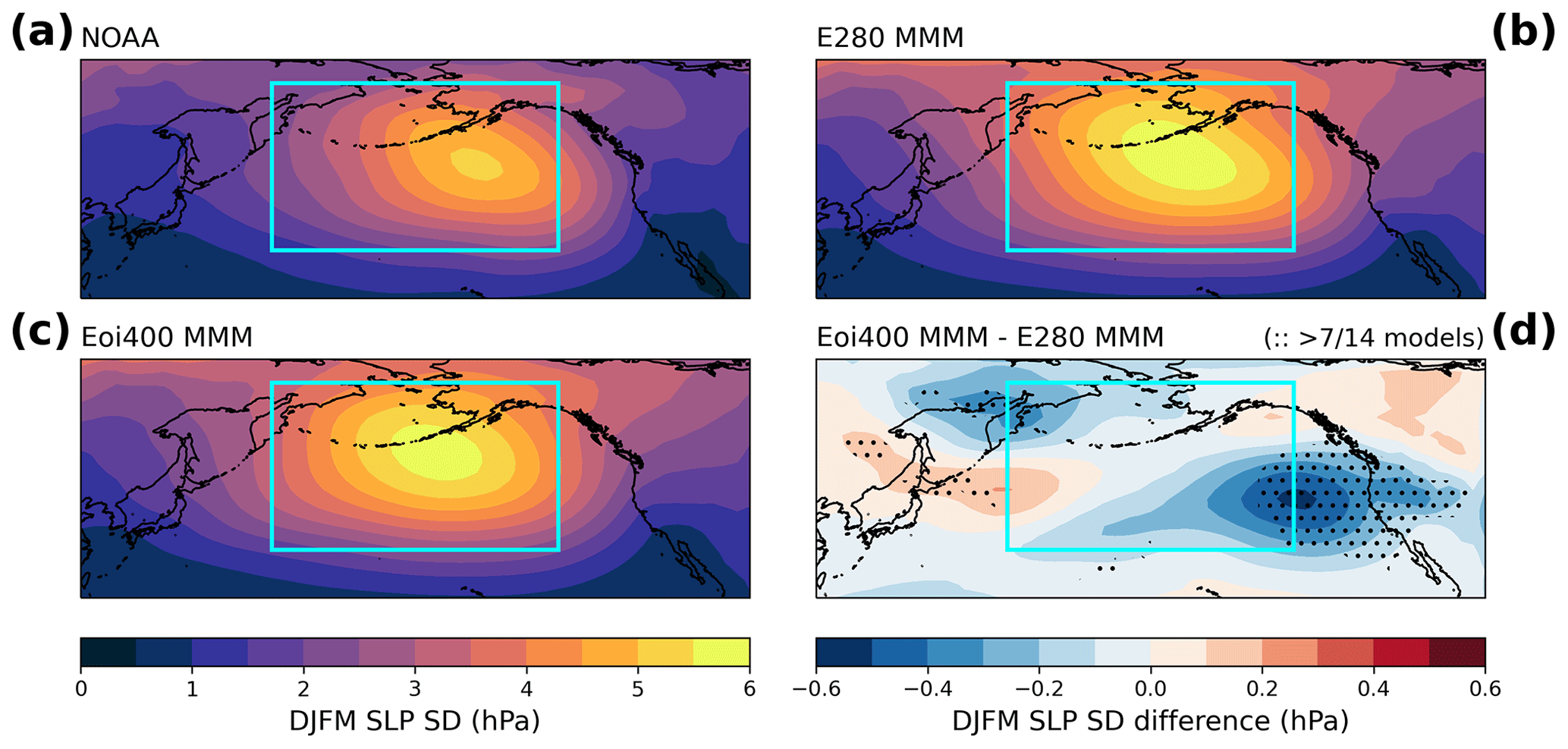
Figure 1Standard deviation (SD) of the DJFM mean sea-level pressure (SLP) for (a) NOAA observations, (b) the E280 multi-model mean (MMM), (c) the Eoi400 MMM, and (d) the difference between the Eoi400 MMM and the E280 MMM. The cyan rectangle indicates the Aleutian Low region. The arcing in panel (d) shows when more than 7 out of 14 models agree with the sign of change.
While the MMM suggests no substantial change in AL variability, a per-model look reveals a variety of responses which are related to the ENSO amplitude change. Figure 2 shows scatter plots of the ENSO amplitude (defined as Niño 3.4 SD) and AL amplitude in the pre-industrial E280 (a), the mid-Pliocene Eoi400 (b), and as the difference between the simulations (c). The ENSO amplitude in the NOAA observations is reproduced well by the E280 ensemble, while the AL amplitude is overestimated by the majority of the models. The Eoi400 ensemble shows a large spread in both ENSO and AL amplitudes compared to the E280. In the E280 and Eoi400, the AL amplitude does not correlate well with the ENSO amplitude (i.e. no statistically significant ensemble correlation, p-value>0.05). However, the change in AL amplitude in the ensemble is related to the change in ENSO amplitude with a statistically significant correlation coefficient of 0.76. Generally, models with slight ENSO change show a similar or increased AL variability in the mid-Pliocene, while the models with substantial ENSO reduction show a similar or reduced AL variability. There is a considerable model spread regarding this relation, though, implying that the change in AL variability is not just related to ENSO change.
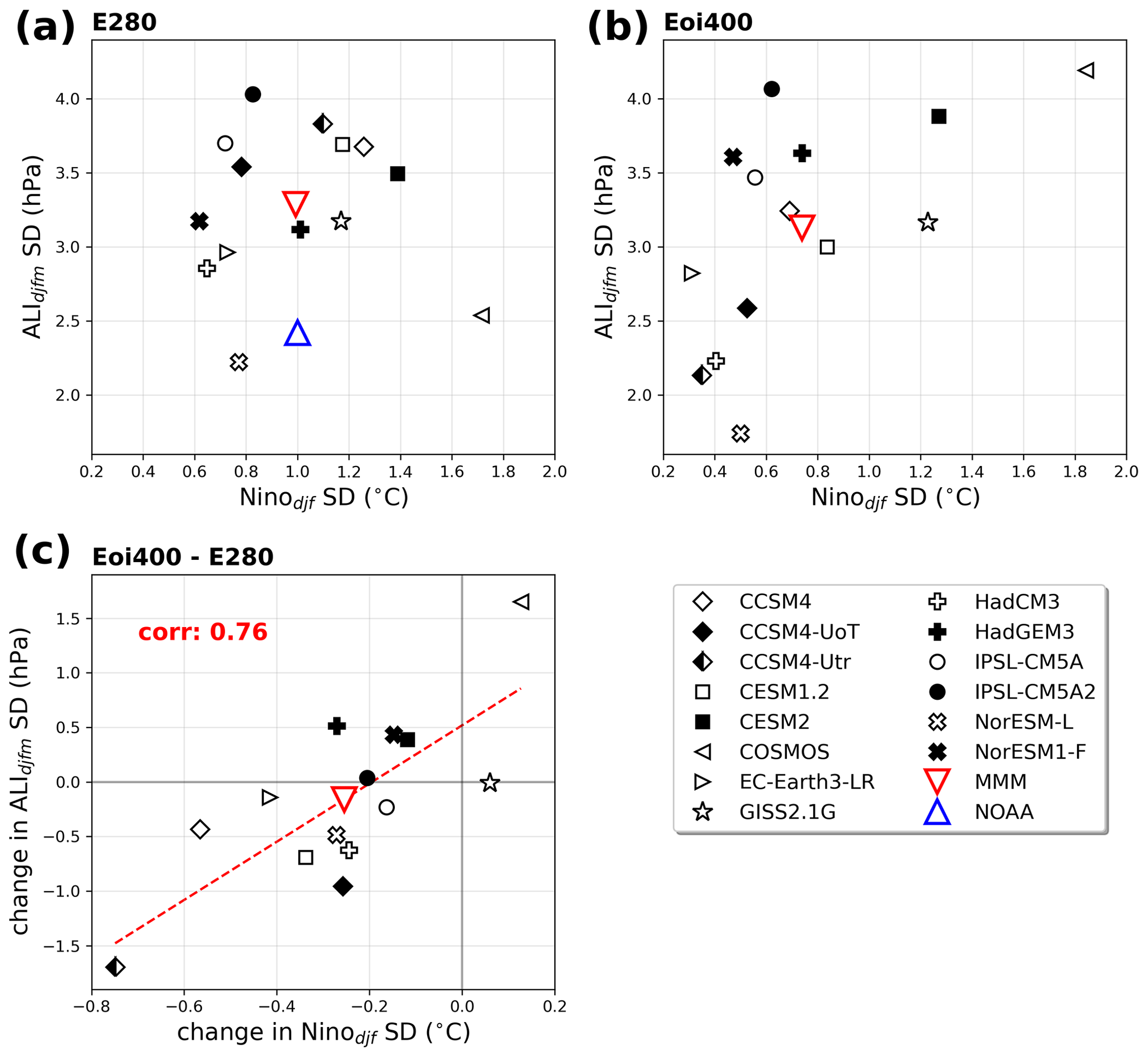
Figure 2Scatter plots of DJF Niño SD versus DJFM AL SD in the E280 (a) and Eoi400 (b) and a scatter plot of Eoi400−E280 differences in Niño SD and AL SD (c). The red triangles show the multi-model mean (MMM), and the blue triangle shows the NOAA observations. The dashed red line in panel (c) is a linear fit through the points, with a significant correlation coefficient of 0.76.
3.2 ENSO teleconnection with the North Pacific atmosphere
Figure 3 shows the linear regression, representing the ENSO–AL teleconnection strength, for the E280 and Eoi400 (a) and the relative change between the two (b). Results per model are included in the Supplement (Fig. S3). The majority of the models overestimate the regression in the pre-industrial when compared to NOAA observations, which is expected, since most models overestimate AL variability, while ENSO variability is similar to observations and correlations are similar too (Fig. S3). The large spread in modelled ENSO–AL teleconnection strength compared to observations is also reported in CMIP5 generation models (e.g. Deser et al., 2017). The MMM shows a similar regression in the pre-industrial and mid-Pliocene. The Eoi400 regression for CCSM4-Utr and EC-Earth3.3 is set to zero because the correlation between ENSO and AL becomes statistically insignificant in the mid-Pliocene simulation (i.e. p-value>0.05). Not doing this would not change the MMM substantially because the correlations are weak nonetheless. Figure 2b shows that the MMM (dashed red line) and median (red line in boxplot) values are slightly positive. However, the confidence intervals around the median (boxplot notches) encompass 0 %, meaning that we cannot statistically speak of an increase in regression. An ensemble end-member is COSMOS, showing the largest increase in regression strength, whereas CCSM4-Utr and EC-Earth3.3 show the largest decrease. The change in regression is weakly but significantly correlated to the change in ENSO and the change in AL across the ensemble (Fig. S4).
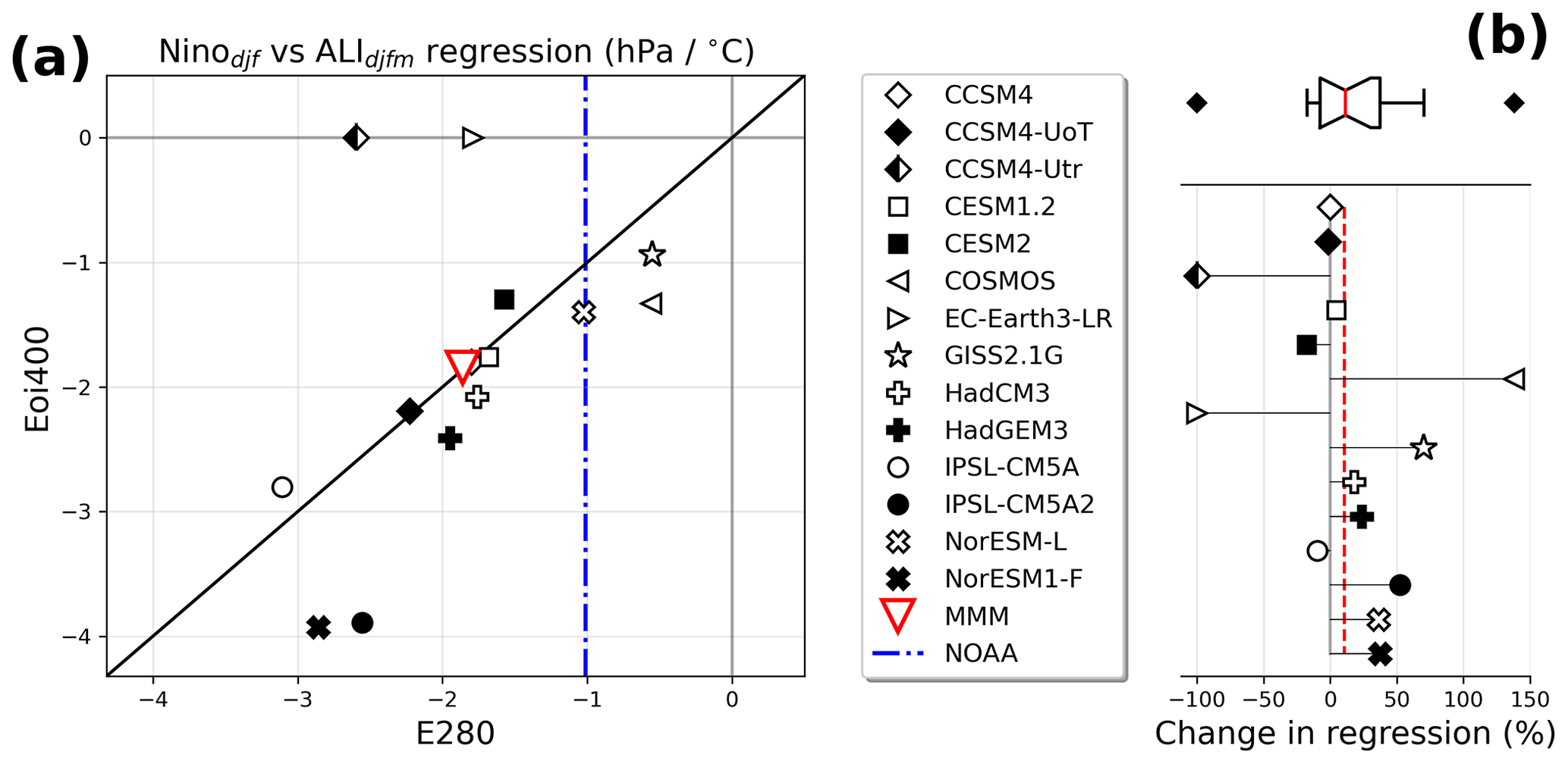
Figure 3(a) Regression (linear slope) between DJF Niño and DJFM AL in the E280 and Eoi400 per model. The red triangle is the multi-model mean (MMM), and the dash-dotted blue line shows the NOAA observations. The Eoi400 value of CCSM4-Utr and EC-Earth3-LR is set to zero because there is no significant correlation between the two variables (i.e. p-value>0.05). (b) Relative change in this regression per model, with the dashed red line indicating the multi-model mean. A boxplot is included (the red line is the median).
Figure 4 shows the E280 MMM regression between the Niño 3.4 index and tropical Pacific precipitation (b) and the WEP precipitation index and SLP in the North Pacific (a). Regressions are only shown when the majority of the models have a statistically significant correlation (i.e. p-value<0.05) in that grid cell. Pre-industrial ENSO variability leads to a strong precipitation signal in the WEP (b; box drawn), and precipitation anomalies in that region lead to a strong SLP signal in the AL region (a; box drawn). The shape and amplitude of the regression patterns look similar to NOAA observations (Fig. S5) and present-day simulations (Williams et al., 2024). Figure 4c shows the change in ENSO–WEP precipitation regression and the change in WEP precipitation–AL regression. The MMM indicates no change in both regressions. It agrees with the previous finding that the ENSO–AL regression does not change, and it shows that this is not because of concealed counteracting changes in the teleconnection processes. Figure 4c also shows that the strong increase in ENSO–AL regression in COSMOS is due to both the ENSO–WEP precipitation and the WEP precipitation–AL regression strengthening. For CCSM4-Utr, the weaker regression is mainly due to the WEP precipitation–AL link weakening, while the weaker regression in EC-Earth3.3 is mainly related to a weakening of the ENSO–WEP precipitation link.
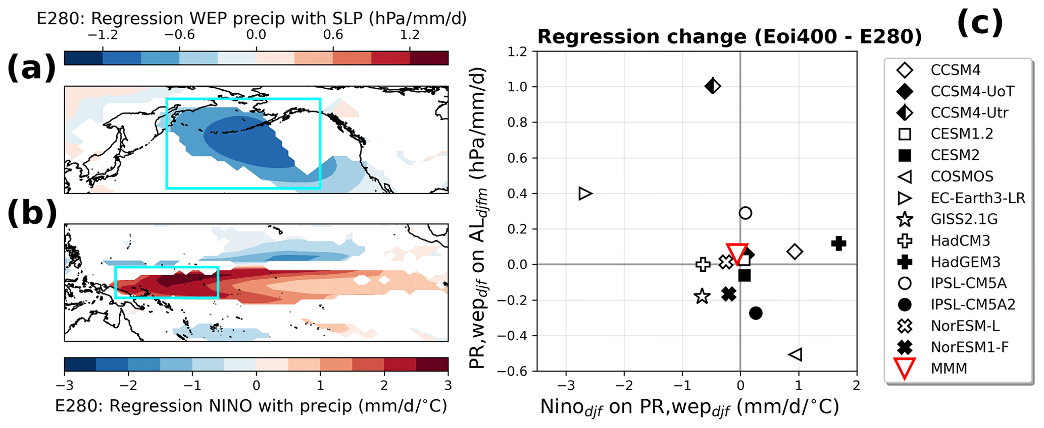
Figure 4(a) E280 multi-model mean (MMM) regression between DJF precipitation in the western equatorial Pacific (WEP) and DJFM SLP in the North Pacific. The cyan rectangle indicates the Aleutian Low region. (b) E280 MMM regression between DJF Niño 3.4 and DJF precipitation. The cyan rectangle indicates the WEP region. For both panels (a) and (b), values are only shown if more than 7 out of 14 models have a statistically significant correlation (p-value<0.05). (c) Scatter plot of Eoi400−E280 change in regression between Niño 3.4 and WEP precipitation versus change in regression between WEP precipitation and AL. The red triangle is the MMM. Regressions in either E280 or Eoi400 are set to 0 when correlations are not statistically significant (i.e. p-value>0.05)
3.3 Separating ENSO- and non-ENSO-related AL variability
We split the AL variability in a part that regresses with ENSO (Niño-regr. part) and a residual following the LRM as explained in Sect. 2. The variances of both parts add up to the total AL variance. Figure 5 shows the Niño-regressing AL variance, the residual AL variance, and the total AL variance for all models and simulations. In the MMM, the Niño-regr. AL variance decreases in the mid-Pliocene, which can be understood, since the ENSO amplitude reduces (Fig. 2c), while the ENSO–AL teleconnection strength does not change (Fig. 3). The AL residual variance does not change in the MMM. The pre-industrial MMM overestimates both parts of the AL variance compared to NOAA observations. It also overestimates the AL variance fraction related to ENSO (0.30 over 0.18), which can be explained, since the MMM regression is overestimated (Fig. 3a), whereas the ENSO amplitude is similar (Fig. 2a). CMIP6 generation models have been shown to generally underestimate the tropical influence on variability in the North Pacific (Zhao et al., 2021), which in this case is true for 4 out 14 models. In the MMM, the fraction of the AL variance related to ENSO decreases from 0.30 to 0.22 in the mid-Pliocene, and 10 out of 14 models agree with that sign of change in variance fraction. For 9 models this is because the ENSO–AL variance decreases. For NorESM1-F the variance fraction decreases because the residual variance increases, while for NorESM-L the variance fraction increases despite a slight reduction in the ENSO-related variance, caused by a stronger reduction in the residual variance. The ENSO-related AL variance is zero for CCSM4-Utr and EC-Earth3.3 because the ENSO–AL regression is set to zero.
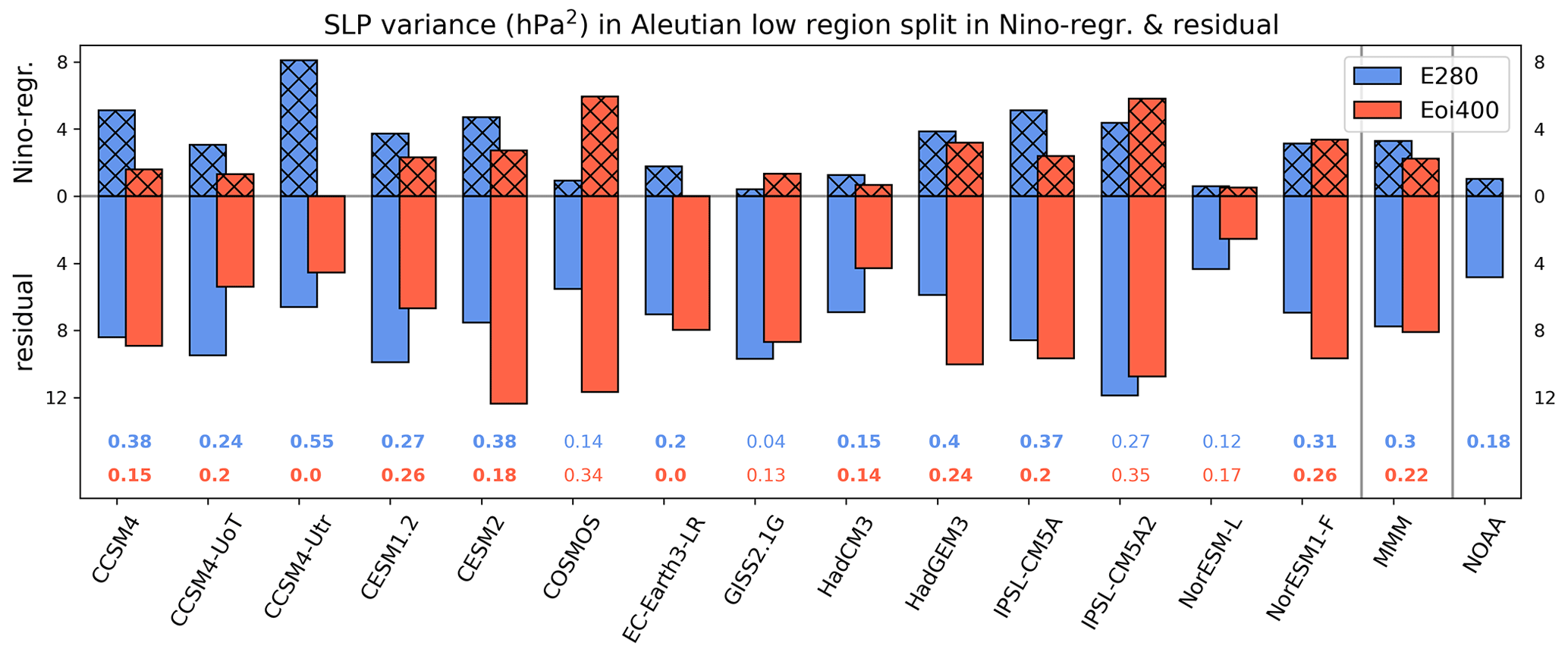
Figure 5Aleutian Low (AL) variance, split (following a linear regression model; LRM) into the AL variance that regresses with Niño (Niño-regr. part; hatched) and the residual AL variance. Results per model for the E280 (blue) and Eoi400 (red), including the multi-model mean (MMM) and the result from NOAA observations. The full bar length represents the total AL variance. Values below are the variance fraction of the Niño-regr. part for E280 (blue, top) and Eoi400 (red, bottom) and are in bold when the variance fraction is lower in the Eoi400 compared to in the E280.
Figure 6 shows the change in the AL amplitude (in terms of SD), split into the part that regresses with ENSO (a) and the residual variability (b) as a function of the change in ENSO amplitude (similar to Fig. 2c). By using the LRM to split the AL variability, we are able to separate the change in AL variability into a part regressing with ENSO where the change is strongly dependent on the change in ENSO variability (corr. coef. of 0.89 over 0.76 for the total AL change; Fig. 2c) and a residual where the change is not related to ENSO change (corr. becomes insignificant). We could expect the ensemble correlation in Fig. 6a to be higher than the ensemble correlation in Fig. 2c if the linear regression between ENSO and the AL were the same between the pre-industrial and the mid-Pliocene. While the MMM regression is largely unchanged (Fig. 3b), the regression change per model can be substantial, implying that the correlation in Fig. 6a is not necessarily higher merely by construct. In the MMM, there is a slight reduction in the ENSO-related AL variability, where 10 of the 14 models agree with that sign of change. The MMM residual AL variability shows no change, with 7 models showing a reduction and 7 showing an increase. The results indicate that the change in total AL variability is primarily driven by a change in ENSO. The residual AL variability does change slightly per model (mean absolute error (MAE) of 0.47 hPa) but on average less than the ENSO-related part (MAE of 0.79 hPa). Since the residual variability is similar and dominates the total AL variability (see Fig. 5), the total AL variability does not seem to change much in the mid-Pliocene along the ensemble, even though ENSO is suppressed.
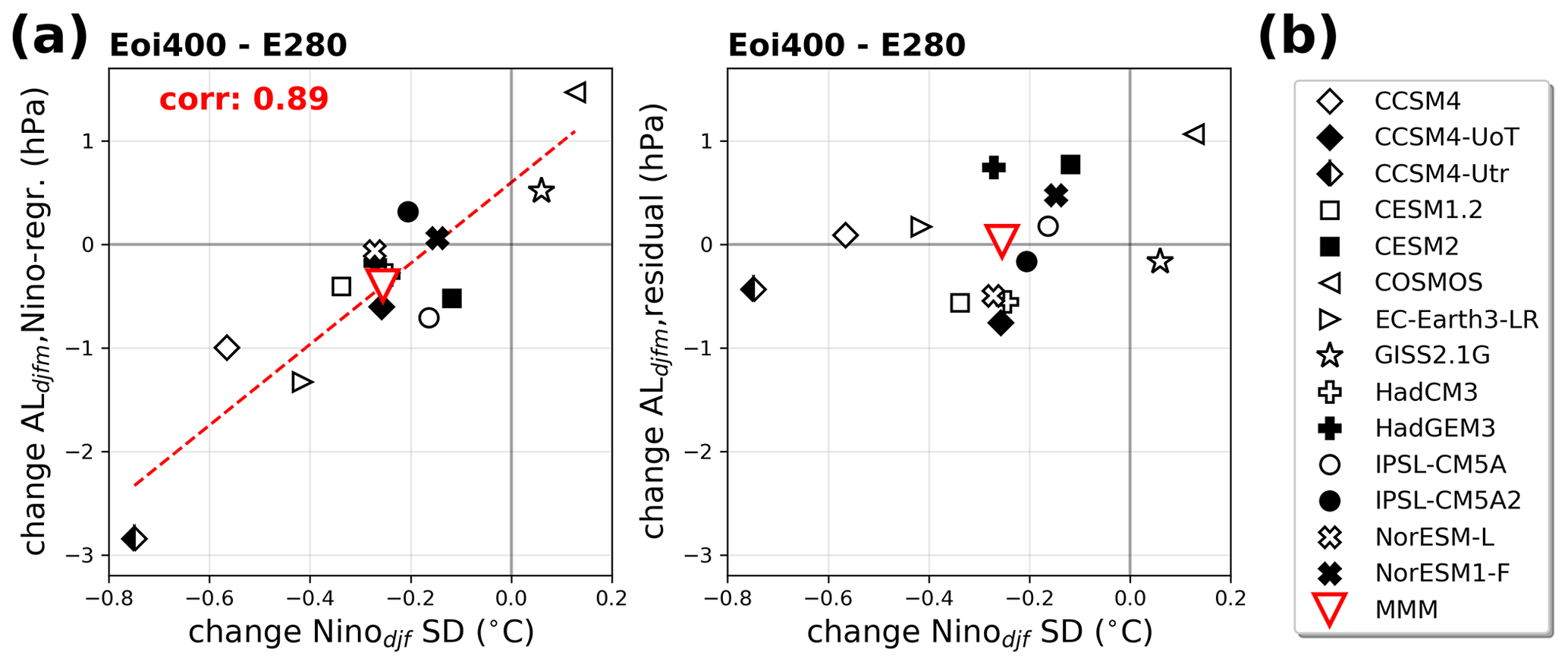
Figure 6Scatter plots of the change in the Eoi400−E280 DJF Niño 3.4 SD versus (a) the change in DJFM AL variability that regresses with Niño (Niño-regr. part) and (b) the change in the residual DJFM AL variability. The red triangle is the multi-model mean (MMM). The dashed red line in panel (a) is a linear fit through the points, with a significant correlation coefficient of 0.89. Multi-model correlation in panel (b) is not statistically significant (i.e. p-value>0.05).
3.4 ENSO and AL variability response in relation to climate sensitivities
Oldeman et al. (2023) use sensitivity simulations to show that CCSM4-Utr's Eoi400 North Pacific variability response is largely dictated by the response to the mid-Pliocene BCs (e.g. closed Arctic gateways, reduced ice sheets) and not by the response to elevated CO2. They hypothesize that this is related to the relatively high sensitivity of the model to the mid-Pliocene BCs compared to its sensitivity to elevated CO2 in terms of global mean temperature response and compared to the PlioMIP2 ensemble. In this section we will investigate this issue in more detail by looking at the ENSO change and the AL change in response to mid-Pliocene boundary conditions and elevated CO2 using sensitivity simulations from a subset of the PlioMIP2 models.
Figure 7a shows the relative change in ENSO variability and AL variability in response to elevated CO2 (in red), mid-Pliocene BCs (in blue), and the “total” mid-Pliocene (i.e. the Eoi400 simulation, in black). There is a clear separation of responses to both forcings. In response to elevated CO2, five out of six simulations show increased AL variability, of which four also show slightly increased ENSO variability. In response to the mid-Pliocene BCs, five out of six simulations show reduced ENSO variability, of which four also show reduced AL variability. It indicates a “tug of war” between the opposite ENSO–AL responses to either mid-Pliocene BCs or elevated CO2, where the total mid-Pliocene (Eoi400) response differs per model, explaining the ensemble spread in Fig. 2c. We argue that whichever forcing “wins” this tug of war is related to the model sensitivity. Figure 7b shows the fraction of the ENSO–AL response which is due to elevated CO2 as a function of the ratio between the model sensitivity to elevated CO2 (i.e. ECS) and the total mid-Pliocene climate sensitivity (ESS). It indicates that a positive relation exists between the ratio and the fraction of the ENSO–AL response due to elevated CO2. The larger the relative model sensitivity to CO2, the more of the ENSO–AL response is related to elevated CO2, and likewise the larger the relative model sensitivity to the mid-Pliocene BCs, the more of the ENSO–AL response is related to the mid-Pliocene BCs. This relationship is not necessarily intuitive; both ECS and ESS are a measure of the annual global mean surface temperature change in response to a certain (combination of) forcing(s), while the fraction of ENSO–AL response is related to the change in ENSO and AL variability in boreal winter due to different forcings. It demonstrates that the (relative) sensitivity of a climate model to a specific forcing is connected with more responses of the climate system than just global mean temperature change.
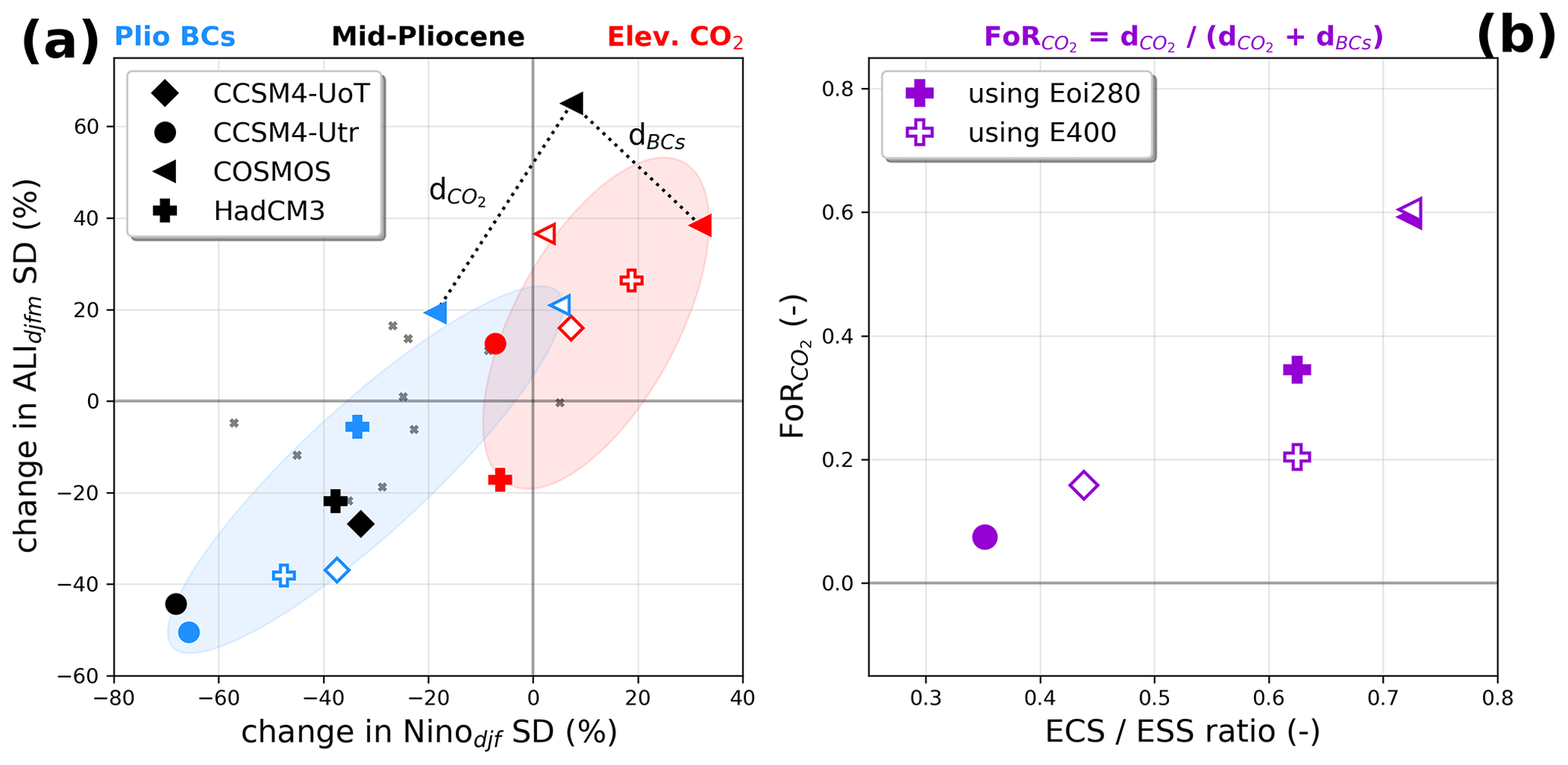
Figure 7(a) Scatter plot of relative change in DJF Niño 3.4 SD vs. relative change in DJFM AL variability for a subset of the PlioMIP2 ensemble and using sensitivity studies. The total mid-Pliocene response is in black (Eoi400−E280), the response to elevated CO2 is in red (white markers for E400−E280 and filled markers for Eoi400−Eoi280), and the response to mid-Pliocene BCs is in blue (white markers for Eoi400−E400 and filled markers for Eoi280−E280). The Eoi400−E280 responses of remaining PlioMIP2 models are denoted by small crosses. Note the different markers used per model compared to previous figures. (b) Fraction of ENSO–AL response (FoR) due to elevated CO2 as a function of the ratio between ECS and ESS. FoR is defined using the distances (in terms of ENSO change and AL change) between the different simulations (see Methods section for details). The ECS and ESS are listed in Table 1.
4.1 Performance of PlioMIP2 with regard to observations and ensemble spread
In this section we discuss the performance of the PlioMIP2 ensemble in assessing changes to the ENSO–AL teleconnection in the mid-Pliocene in terms of comparing pre-industrial results with NOAA observations and the within-ensemble performance. The PlioMIP2 models are generally better at reproducing the amplitude of ENSO variability compared to NOAA observations (Fig. 2a; for more detail see Oldeman et al., 2021). The model that best reproduces the NOAA observations in the pre-industrial is NorESM-L, which also shows changes to ENSO and AL variability in the mid-Pliocene that are very close to the MMM (Fig. 2c). Most models overestimate the ENSO–AL regression strength (Fig. 3a), which is not surprising considering that the amplitude of ENSO variability is similar, that the amplitude of AL variability is overestimated, and that the correlation coefficient between ENSO and AL indices is similar for most E280 simulations and NOAA observations (Fig. S3). The shape and amplitude of the pre-industrial MMM ENSO–precipitation relation (Fig. 4b) is similar to NOAA observations and is similar to the response in present-day simulations with higher-resolution models (Williams et al., 2024). The fraction of AL variance related to ENSO is overestimated in the E280 MMM compared to NOAA observations (Fig. 5). An important feature is that the AL variance fraction of the residual is larger than the fraction of AL variance related to ENSO, which is captured by all E280 simulations except for CCSM4-Utr. Finally, it should be noted that any discrepancies between NOAA observations and the pre-industrial simulations can also arise from the fact that we are comparing equilibrated pre-industrial simulations with historical observations. Even though the observations have been detrended, there will be an anthropogenic signal present which is absent from the simulations considered.
In terms of ENSO and AL change (e.g. Figs. 2c, 6, and 7a), the clear end-members of the ensemble are CCSM4-Utr on the one hand, showing the largest reduction in ENSO and AL variability, and COSMOS on the other hand, showing the largest increase in ENSO and AL variability. Our results show that this spread in responses is related to the relative model sensitivities of these two models to either the Pliocene BCs or the elevated CO2 (Fig. 7b). COSMOS is one of the coarsest models in terms of ocean and atmosphere resolution (Table 1). Its E280 simulation performs well in terms of AL variability compared to NOAA observations, but the ENSO variability is greatly overestimated. Williams et al. (2024) show improved simulation of the ENSO–AL teleconnection with increased model resolution. CCSM4-Utr, on the other hand, performs well in terms of ENSO variability but substantially overestimates AL variability compared to NOAA observations. However, as shown in Oldeman et al. (2023), the patterns of North Pacific atmospheric variability (i.e. the spatial patterns, amplitudes, and variance fractions of the PNA pattern and NPO) are very well reproduced, even though the total amplitude is overestimated.
4.2 Changes in the residual Aleutian Low variability
We find that, in the mid-Pliocene, a change in AL variability is related to a change in ENSO variability (Fig. 2c). This relation originates from a change in AL variability which linearly covaries with the ENSO signal (Fig. 6a). The residual AL variability also changes, but the change is model-dependent and not related to a change in ENSO variability (Fig. 6b). The change in residual AL variability is also not related to a change in residual WEP precipitation (Fig. S6). In this section, we explore the residual Aleutian Low variability in more detail and hypothesize what its change might be related to.
4.2.1 Nonlinear ENSO interactions
We separated the AL variability in an ENSO-related and residual part following an LRM. This implies that the residual AL variability will also contain nonlinear ENSO contributions. Any nonlinear atmospheric response to ENSO SST variability can be regarded as a sum of nonlinear responses to a linear ENSO and of linear responses to a nonlinear ENSO (Frauen et al., 2014). ENSO variability is known to be nonlinear, originating from diversity in ENSO events and from asymmetry in pattern and duration between El Niño and La Niña events (e.g. Ashok et al., 2007; Yeh et al., 2009; Okumura, 2019; Cai et al., 2021). In the PlioMIP2 MMM, both the skewness of the Niño 3.4 index and the ratio between central Pacific and eastern Pacific ENSO events are unchanged compared to the pre-industrial (Oldeman et al., 2021). However, there is a considerable model spread, both in terms of change in the mid-Pliocene and of differences in observations. The atmospheric response to ENSO variability is complex and known to encompass nonlinearity originating from a variety of factors (e.g. Yeh et al., 2018; Domeisen et al., 2019; Jiménez-Esteve and Domeisen, 2019), the main factor being the nonlinear relationship between ENSO variability and tropical precipitation (Deser and Wallace, 1990). This nonlinear ENSO–precipitation relationship changes in a warming climate (Yun et al., 2021). Only about half of the PlioMIP2 models capture the nonlinear nature of the ENSO–precipitation relationship (Pontes et al., 2022). In conclusion, since there is considerable model spread in changes in both ENSO skewness and kurtosis (Oldeman et al., 2021) and in the ENSO–precipitation relation (Pontes et al., 2022, and Fig. 4c of this study), nonlinearity in the atmospheric response to ENSO could explain some of the residual AL variability, but the exact contribution is likely model-dependent. Considering ENSO diversity and its nonlinear interactions, removing ENSO influence from North Pacific variability using linear regression might not always be the best option (Zhao et al., 2021). Improving the separation of (nonlinear) ENSO influence from the North Pacific variability response in PlioMIP2 is outside the scope of this work.
4.2.2 Stochastic internal variability
Apart from the deterministic link with the tropics via the atmospheric bridge, AL variability is forced by internal stochastic variability originating from the extra-tropical atmosphere (Di Lorenzo et al., 2013; Newman et al., 2016). Indeed, the existence of modes of winter variability in the Northern Hemisphere atmosphere can largely be explained by internal or stochastic variability (Branstator, 2002; Branstator and Selten, 2009). Idealized models with no ENSO variability or ocean dynamics show that the dominant SLP variability in the North Pacific is located in the Aleutian Low region, resulting from internal atmospheric dynamics (Pierce, 2001; Alexander, 2010). Modes of variability in the Northern Hemisphere extratropics such as the NAO and Arctic Oscillation, but also Pacific modes such as the PNA pattern, are related to variability in the jet streams (e.g. Ambaum et al., 2001; Linkin and Nigam, 2008) and are related to each other through a circumglobal teleconnection (e.g. Barnston and Livezey, 1987; Branstator, 2002). It suggests that changes in atmospheric circulation originating from the mid-Pliocene boundary conditions (e.g. the reduced Greenland ice sheet) can ultimately lead to changes in atmospheric variability in the North Pacific. Research on the Last Glacial Maximum atmosphere indeed shows a distorted pattern of variability in the North Pacific related to jet stream changes originating from changes in ice sheet extent and not related to ENSO (Hu et al., 2020). Apart from the internal atmospheric dynamics, North Pacific winter atmospheric variability has been linked to variations in sea-ice extent and North Pacific SSTs (e.g. Linkin and Nigam, 2008; Hurwitz et al., 2012; Simon et al., 2022). Across the PlioMIP2 ensemble, changes in mid-Pliocene sea-ice extent (via De Nooijer et al., 2020) or North Pacific SSTs do not relate to changes in the residual AL variability (Fig. S7). Garfinkel et al. (2020) show that patterns in the North Pacific wintertime atmosphere can be explained by a sum of forcings related to the land–sea contrast, heat fluxes in the ocean, and topography. In the mid-Pliocene simulations, the land–sea contrast is different due to changes in the land–sea mask and in vegetation and lakes, and the topography is different, albeit not substantially. Differences in ocean heat fluxes could originate from the closure of the Arctic gateways, which has been shown to cause a strengthening of the mid-Pliocene AMOC (Weiffenbach et al., 2023). Changes in the AMOC and changes in the Arctic surface temperatures do not relate to changes in the residual AL variability (Fig. S7). Considering that every climate model will have different sensitivities of its internal atmospheric variability response to the different mid-Pliocene boundary conditions, it might be hard, if not impossible, to find one common driver that is able to explain changes to the residual AL variability in the mid-Pliocene.
4.3 Synthesis of tropical–North Pacific variability in PlioMIP2
In the last part of the Discussion, we present a synthesis of the results presented in this paper on the mid-Pliocene changes in North Pacific atmosphere variability combined with other published results using PlioMIP2 data, specifically regarding tropical–North Pacific variability (Oldeman et al., 2021; Pontes et al., 2022) and Indo-Pacific tropical mean climate (Han et al., 2021; Ren et al., 2023; Zhang et al., 2024). Figure 8 presents a summary view of the interactions of mid-Pliocene tropical and extratropical variability and mean state changes according to the PlioMIP2 MMM.
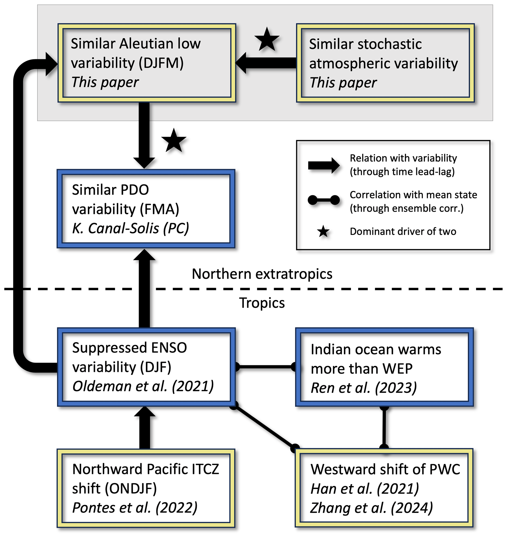
Figure 8Summary view of interactions and mechanisms of mid-Pliocene tropical and extratropical variability in the North Pacific according to the PlioMIP2 multi-model mean. Blue boxes are ocean features, and yellow boxes are atmosphere features. Black arrows are relationships with variability of which we know the direction of influence (through lead–lag), black connector lines are relationships with the mean state (through ensemble correlations) of which we do not know the direction, and ★ indicates the dominant driver out of the two main drivers. The grey box indicates features primarily assessed in the present study. PDO results are obtained from Katya Canal-Solis and Julia Tindall through personal communications (2024) (PC).
In PlioMIP2, ENSO variability is suppressed (Oldeman et al., 2021), which is caused by a series of off-equatorial processes triggered by a northward displacement of the Pacific ITCZ (Pontes et al., 2022). In the tropical Indo-Pacific mean climate, the rising branch of the Pacific Walker circulation (PWC) is shifted westwards, both in the annual mean (Han et al., 2021) and in boreal winter (Zhang et al., 2024). Furthermore, the Indian Ocean, the Maritime Continent, and the WEP warm, but the Indian Ocean warms more than the WEP (Ren et al., 2023). We hypothesize that the westward shift of the PWC, the Indo-Pacific warming asymmetry, and the ENSO suppression are related, and we find that there is indeed a significant ensemble correlation between the change in these three variables (Fig. S8). Explaining the direction and causality of these links is out of the scope of this work.
In the present-day extratropics, ENSO forces AL variability and PDO variability, AL variability is also forced by internal stochastic variability which is dominant, and PDO variability is also forced by the AL variability which is dominant over ENSO forcing (e.g. Trenberth and Hurrell, 1994; Di Lorenzo et al., 2013; Newman et al., 2016). In PlioMIP2, the amplitude of PDO variability is similar to the pre-industrial, and ENSO leads PDO variability with a similar correlation (Fig. S9). In this study, we find that the amplitude of AL variability is also similar and that the leading regression with ENSO is largely unchanged. Furthermore, the internal stochastic atmospheric variability forcing AL variability is similar. So, despite ENSO being suppressed, AL variability is similar because the dominant driver (internal variability) is similar as in the pre-industrial. Likewise, PDO variability is similar despite ENSO being suppressed, because the dominant driver (AL variability) is similar to that in the pre-industrial. We also confirm that, in PlioMIP2, AL variability leads the PDO, with a higher correlation than with ENSO (Fig. S1).
The benefit of the view presented in Fig. 8 is that we are able to combine previously published results on changes to (extra-)tropical variability and mean climate in PlioMIP2 to the results of this study. It provides a view that shows the PlioMIP2 MMM changes tendency, with which a majority of the models (generally) agree. A weakness, however, is that information on spread in the ensemble is not included. For example, while a clear majority of the PlioMIP2 ensemble shows a westward shift in the PWC (11 out of 13; Han et al., 2021) and reduced ENSO variability (15 out of 17; Oldeman et al., 2021), the change in AL variability is similar according to the MMM, but most models show a substantial change which is either positive or negative. In this specific example, we have described these opposing responses as a “tug of war” between different responses to different boundary conditions (Fig. 7). In conclusion, the MMM view can provide useful information, but it can conceal a range of changes in opposing directions that can relate to the amplitude of a more obvious change in one direction.
The mid-Pliocene is the most recent geological period with similar atmospheric CO2 concentrations to the present day and similar surface temperatures to those projected at the end of this century for a moderate warming scenario. According to the mid-Pliocene modelling ensemble PlioMIP2, ENSO variability was suppressed (Oldeman et al., 2021; Pontes et al., 2022). In this study, we investigate how variability in the North Pacific atmosphere responds to a suppressed ENSO in the warm mid-Pliocene climate according to the PlioMIP2 ensemble.
We find limited changes to the variability in the Aleutian Low (AL) in the MMM compared to the pre-industrial. Models with a similar ENSO variability show an increase in AL variability in the mid-Pliocene, while models with a suppressed ENSO variability also show suppressed AL variability. The majority of the ensemble shows relatively little change in ENSO–AL teleconnection strength. We separate the AL variability into a part that regresses with ENSO and into a residual, which mainly represents internal variability. We find, agreeing with observations, that most of the AL variance is explained by the residual and that a smaller part is explained by the variability that regresses with ENSO (in both climates). The change in ENSO-related AL variability is strongly related to the change in ENSO itself, while the change in the residual AL variability is not related to ENSO change. A brief investigation does not reveal one change that is able to explain changes in the residual AL variability for the whole ensemble. We find that the specific change in ENSO and AL variability depends on the relative model sensitivity either to elevated CO2 or to the other mid-Pliocene boundary conditions, which include closed Arctic gateways and reduced ice sheet extent. Specifically, models that are relatively sensitive to elevated CO2 generally show ENSO variability that is similar or increased compared to the pre-industrial and AL variability that is increased, while models that are relatively sensitive to the mid-Pliocene boundary conditions generally show reduced ENSO and similar or reduced AL variability.
We present a summary perspective of tropical–North Pacific variability in PlioMIP2, combining our results with the literature. Changes in the tropical Pacific mean climate result in a suppression of the mid-Pliocene ENSO variability, but since the dominant internal variability in the North Pacific extratropics is largely unchanged, both AL variability in the atmosphere and PDO variability in the ocean are similar to the pre-industrial and are not necessarily suppressed. Evaluating the effect of past climate boundary conditions, including changes to ice sheets and Arctic gateways, on the internal variability of the extratropical atmosphere is a topic for future research.
While the mid-Pliocene is not a perfect analogue for near-future climate, investigating atmosphere–ocean interactions in the mid-Pliocene provides a useful view of the functioning of the Earth system under different forcings. Our results show that teleconnections of a suppressed ENSO in a warmer past climate are quite robust. Furthermore, we are able to explain how suppressed ENSO variability does not have to lead to a suppression of its connected modes of variability in the North Pacific. Lastly, we demonstrate that, in addition to equilibrium climate sensitivity, we need Earth system sensitivity in order to explain the spread in simulated climate variability responses in the mid-Pliocene.
Codes (Python and Jupyter notebooks) for pre-processing the data and for analysing and generating the figures are available on GitHub and published on Zenodo (https://doi.org/10.5281/zenodo.10817269; Oldeman, 2024). The PlioMIP2 model data used in this work are available from the PlioMIP2 database upon request from Alan M. Haywood (a.m.haywood@leeds.ac.uk). PlioMIP2 data from CESM2, EC-Earth3.3, NorESM1-F, IPSL-CM6A, GISS2.1G, and HadGEM3 can be obtained from the Earth System Grid Federation (https://esgf-node.llnl.gov/search/cmip6/, ESGF, 2024). NOAA Extended Reconstructed SST V5 data are provided by the NOAA PSL, Boulder, Colorado, USA, on their website at https://psl.noaa.gov/data/gridded/data.noaa.ersst.v5.html (Slivinski et al., 2021). NOAA/CIRES/DOE 20th Century Reanalysis (V3) data are provided by the NOAA PSL, Boulder, Colorado, USA, on their website at https://psl.noaa.gov/data/gridded/data.20thC_ReanV3.html (Huang et al., 2017).
The supplement related to this article is available online at: https://doi.org/10.5194/esd-15-1037-2024-supplement.
All authors contributed to the ideas leading to this work. AMO performed the analyses, made the figures, and wrote the paper. MLJB, ASvdH, FMS, and HAD provided comments on the paper.
The contact author has declared that none of the authors has any competing interests.
Publisher's note: Copernicus Publications remains neutral with regard to jurisdictional claims made in the text, published maps, institutional affiliations, or any other geographical representation in this paper. While Copernicus Publications makes every effort to include appropriate place names, the final responsibility lies with the authors.
This work was carried out under the programme of the Netherlands Earth System Science Centre (NESSC), financially supported by the Ministry of Education, Culture and Science (OCW grant no. 024.002.001). We thank the PlioMIP2 climate modelling groups for producing and making available their model output. The authors would like to thank Zixuan Han for providing PlioMIP2 data on the Pacific Walker circulation and Katya Canal-Solis and Julia Tindall for providing unpublished results on the PlioMIP2 Pacific Decadal Oscillation. The authors thank the two anonymous reviewers for feedback on the first version of the paper.
This research has been supported by the Netherlands Earth System Science Centre (grant no. 024.002.001).
This paper was edited by Claudia Timmreck and reviewed by two anonymous referees.
Alexander, M.: Extratropical air-sea interaction, sea surface temperature variability, and the Pacific Decadal Oscillation, in: Geophysical Monograph Series, vol. 189, edited by: Sun, D.-Z. and Bryan, F., American Geophysical Union, Washington, D. C., 123–148, https://doi.org/10.1029/2008GM000794, 2010. a
Alexander, M. A., Bladé, I., Newman, M., Lanzante, J. R., Lau, N. C., and Scott, J. D.: The atmospheric bridge: The influence of ENSO teleconnections on air-sea interaction over the global oceans, J. Climate, 15, 2205–2231, https://doi.org/10.1175/1520-0442(2002)015<2205:TABTIO>2.0.CO;2, 2002. a, b
Ambaum, M. H., Hoskins, B. J., and Stephenson, D. B.: Arctic Oscillation or North Atlantic Oscillation?, J. Climate, 14, 3495–3507, https://doi.org/10.1175/1520-0442(2001)014<3495:AOONAO>2.0.CO;2, 2001. a
Ashok, K., Behera, S. K., Rao, S. A., Weng, H., and Yamagata, T.: El Niño Modoki and its possible teleconnection, J. Geophys. Res., 112, C11007, https://doi.org/10.1029/2006JC003798, 2007. a
Baatsen, M. L. J., von der Heydt, A. S., Kliphuis, M. A., Oldeman, A. M., and Weiffenbach, J. E.: Warm mid-Pliocene conditions without high climate sensitivity: the CCSM4-Utrecht (CESM 1.0.5) contribution to the PlioMIP2, Clim. Past, 18, 657–679, https://doi.org/10.5194/cp-18-657-2022, 2022. a
Barnston, A. G. and Livezey, R. E.: Classification, Seasonality and Persistence of Low-Frequency Atmospheric Circulation Patterns, Mon. Weather Rev., 115, 1083–1126, https://doi.org/10.1175/1520-0493(1987)115<1083:CSAPOL>2.0.CO;2, 1987. a, b
Beobide-Arsuaga, G., Bayr, T., Reintges, A., and Latif, M.: Uncertainty of ENSO-amplitude projections in CMIP5 and CMIP6 models, Clim. Dynam., 56, 3875–3888, https://doi.org/10.1007/s00382-021-05673-4, 2021. a
Berntell, E., Zhang, Q., Li, Q., Haywood, A. M., Tindall, J. C., Hunter, S. J., Zhang, Z., Li, X., Guo, C., Nisancioglu, K. H., Stepanek, C., Lohmann, G., Sohl, L. E., Chandler, M. A., Tan, N., Contoux, C., Ramstein, G., Baatsen, M. L. J., von der Heydt, A. S., Chandan, D., Peltier, W. R., Abe-Ouchi, A., Chan, W.-L., Kamae, Y., Williams, C. J. R., Lunt, D. J., Feng, R., Otto-Bliesner, B. L., and Brady, E. C.: Mid-Pliocene West African Monsoon rainfall as simulated in the PlioMIP2 ensemble, Clim. Past, 17, 1777–1794, https://doi.org/10.5194/cp-17-1777-2021, 2021. a
Branstator, G.: Circumglobal Teleconnections, the Jet Stream Waveguide, and the North Atlantic Oscillation, J. Climate, 15, 1893–1910, https://doi.org/10.1175/1520-0442(2002)015<1893:CTTJSW>2.0.CO;2, 2002. a, b
Branstator, G. and Selten, F.: “Modes of Variability” and Climate Change, J. Climate, 22, 2639–2658, https://doi.org/10.1175/2008JCLI2517.1, 2009. a
Brierley, C. M.: Interannual climate variability seen in the Pliocene Model Intercomparison Project, Clim. Past, 11, 605–618, https://doi.org/10.5194/cp-11-605-2015, 2015. a
Burke, K. D., Williams, J. W., Chandler, M. A., Haywood, A. M., Lunt, D. J., and Otto-Bliesner, B. L.: Pliocene and Eocene provide best analogs for near-future climates, P. Natl. Acad. Sci. USA, 115, 13288–13293, https://doi.org/10.1073/pnas.1809600115, 2018. a
Cai, W., Wu, L., Lengaigne, M., Li, T., McGregor, S., Kug, J. S., Yu, J. Y., Stuecker, M. F., Santoso, A., Li, X., Ham, Y. G., Chikamoto, Y., Ng, B., McPhaden, M. J., Du, Y., Dommenget, D., Jia, F., Kajtar, J. B., Keenlyside, N., Lin, X., Luo, J. J., Martín-Rey, M., Ruprich-Robert, Y., Wang, G., Xie, S. P., Yang, Y., Kang, S. M., Choi, J. Y., Gan, B., Kim, G. I., Kim, C. E., Kim, S., Kim, J. H., and Chang, P.: Pantropical climate interactions, Science, 363, eaav4236, https://doi.org/10.1126/science.aav4236, 2019. a
Cai, W., Santoso, A., Collins, M., Dewitte, B., Karamperidou, C., Kug, J.-S., Lengaigne, M., McPhaden, M. J., Stuecker, M. F., Taschetto, A. S., Timmermann, A., Wu, L., Yeh, S.-W., Wang, G., Ng, B., Jia, F., Yang, Y., Ying, J., Zheng, X.-T., Bayr, T., Brown, J. R., Capotondi, A., Cobb, K. M., Gan, B., Geng, T., Ham, Y.-G., Jin, F.-F., Jo, H.-S., Li, X., Lin, X., McGregor, S., Park, J.-H., Stein, K., Yang, K., Zhang, L., and Zhong, W.: Changing El Niño–Southern Oscillation in a warming climate, Nature Reviews Earth & Environment, 2, 628–644, https://doi.org/10.1038/s43017-021-00199-z, 2021. a, b, c
Callahan, C. W., Chen, C., Rugenstein, M., Bloch-Johnson, J., Yang, S., and Moyer, E. J.: Robust decrease in El Niño/Southern Oscillation amplitude under long-term warming, Nat. Clim. Change, 11, 752–757, https://doi.org/10.1038/s41558-021-01099-2, 2021. a
Chan, W.-L. and Abe-Ouchi, A.: Pliocene Model Intercomparison Project (PlioMIP2) simulations using the Model for Interdisciplinary Research on Climate (MIROC4m), Clim. Past, 16, 1523–1545, https://doi.org/10.5194/cp-16-1523-2020, 2020. a
Chandan, D. and Peltier, W. R.: Regional and global climate for the mid-Pliocene using the University of Toronto version of CCSM4 and PlioMIP2 boundary conditions, Clim. Past, 13, 919–942, https://doi.org/10.5194/cp-13-919-2017, 2017. a
Chen, S., Chen, W., Wu, R., Yu, B., and Graf, H.-F.: Potential Impact of Preceding Aleutian Low Variation on El Niño–Southern Oscillation during the Following Winter, J. Climate, 33, 3061–3077, https://doi.org/10.1175/JCLI-D-19-0717.1, 2020. a
Chen, Z., Gan, B., Wu, L., and Jia, F.: Pacific-North American teleconnection and North Pacific Oscillation: historical simulation and future projection in CMIP5 models, Clim. Dynam., 50, 4379–4403, https://doi.org/10.1007/s00382-017-3881-9, 2018. a, b
Chiang, J. C. H. and Vimont, D. J.: Analogous Pacific and Atlantic Meridional Modes of Tropical Atmosphere–Ocean Variability, J. Climate, 17, 4143–4158, https://doi.org/10.1175/JCLI4953.1, 2004. a
de la Vega, E., Chalk, T. B., Wilson, P. A., Bysani, R. P., and Foster, G. L.: Atmospheric CO2 during the Mid-Piacenzian Warm Period and the M2 glaciation, Sci. Rep.-UK, 10, 9–16, https://doi.org/10.1038/s41598-020-67154-8, 2020. a
de Nooijer, W., Zhang, Q., Li, Q., Zhang, Q., Li, X., Zhang, Z., Guo, C., Nisancioglu, K. H., Haywood, A. M., Tindall, J. C., Hunter, S. J., Dowsett, H. J., Stepanek, C., Lohmann, G., Otto-Bliesner, B. L., Feng, R., Sohl, L. E., Chandler, M. A., Tan, N., Contoux, C., Ramstein, G., Baatsen, M. L. J., von der Heydt, A. S., Chandan, D., Peltier, W. R., Abe-Ouchi, A., Chan, W.-L., Kamae, Y., and Brierley, C. M.: Evaluation of Arctic warming in mid-Pliocene climate simulations, Clim. Past, 16, 2325–2341, https://doi.org/10.5194/cp-16-2325-2020, 2020. a, b, c
Deser, C. and Wallace, J. M.: Large-Scale Atmospheric Circulation Features of Warm and Cold Episodes in the Tropical Pacific, J. Climate, 3, 1254–1281, https://doi.org/10.1175/1520-0442(1990)003<1254:LSACFO>2.0.CO;2, 1990. a, b
Deser, C., Simpson, I. R., McKinnon, K. A., and Phillips, A. S.: The Northern Hemisphere Extratropical Atmospheric Circulation Response to ENSO: How Well Do We Know It and How Do We Evaluate Models Accordingly?, J. Climate, 30, 5059–5082, https://doi.org/10.1175/JCLI-D-16-0844.1, 2017. a, b
Di Lorenzo, E. and Mantua, N.: Multi-year persistence of the 2014/15 North Pacific marine heatwave, Nat. Clim. Change, 6, 1042–1047, https://doi.org/10.1038/nclimate3082, 2016. a
Di Lorenzo, E., Combes, V., Keister, J., Strub, P. T., Thomas, A., Franks, P., Ohman, M., Furtado, J., Bracco, A., Bograd, S., Peterson, W., Schwing, F., Chiba, S., Taguchi, B., Hormazabal, S., and Parada, C.: Synthesis of Pacific Ocean Climate and Ecosystem Dynamics, Oceanography, 26, 68–81, https://doi.org/10.5670/oceanog.2013.76, 2013. a, b, c
Domeisen, D. I., Garfinkel, C. I., and Butler, A. H.: The Teleconnection of El Niño Southern Oscillation to the Stratosphere, Rev. Geophys., 57, 5–47, https://doi.org/10.1029/2018RG000596, 2019. a, b
Dowsett, H., Dolan, A., Rowley, D., Moucha, R., Forte, A. M., Mitrovica, J. X., Pound, M., Salzmann, U., Robinson, M., Chandler, M., Foley, K., and Haywood, A.: The PRISM4 (mid-Piacenzian) paleoenvironmental reconstruction, Clim. Past, 12, 1519–1538, https://doi.org/10.5194/cp-12-1519-2016, 2016. a, b, c
ESGF: CMIP6 data, ESGF [data set], https://esgf-node.llnl.gov/search/cmip6/, last access: 6 August 2024. a
Eyring, V., Gillet, N., Achuta Rao, K., Barimalala, R., Barreiro Parrillo, M., Bellouin, N., Cassou, C., Durack, P., Kosaka, Y., McGregor, S., Min, S., Morgenstern, O., and Sun, Y.: Human Influence on the Climate System (Chap. 3), in: Climate Change 2021: The Physical Science Basis. Contribution of Working Group I to the Sixth Assessment Report of the Intergovernmental Panel on Climate Change, edited by: Masson-Delmotte, V., Zhai, P., Pirani, A., Connors, S. L., Péan, C., Berger, S., Caud, N., Chen, Y., Goldfarb, L., Gomis, M. I., Huang, M., Leitzell, K., Lonnoy, E., Matthews, J. B. R., Maycock, T. K., Waterfield, T., Yelekçi, O., Yu, R., and Zhou, B., Cambridge University Press, 423–552, https://doi.org/10.1017/9781009157896.005, 2021. a, b
Fedorov, A. V., Dekens, P. S., McCarthy, M., Ravelo, A. C., DeMenocal, P. B., Barreiro, M., Pacanowski, R. C., and Philander, S. G.: The pliocene paradox (mechanisms for a permanent El Niño), Science, 312, 1485–1489, https://doi.org/10.1126/science.1122666, 2006. a
Feng, R., Otto-Bliesner, B. L., Brady, E. C., and Rosenbloom, N.: Increased Climate Response and Earth System Sensitivity From CCSM4 to CESM2 in Mid-Pliocene Simulations, J. Adv. Model. Earth Sy., 12, e2019MS002033, https://doi.org/10.1029/2019MS002033, 2020. a, b, c
Feng, R., Bhattacharya, T., Otto-Bliesner, B. L., Brady, E. C., Haywood, A. M., Tindall, J. C., Hunter, S. J., Abe-Ouchi, A., Chan, W.-L., Kageyama, M., Contoux, C., Guo, C., Li, X., Lohmann, G., Stepanek, C., Tan, N., Zhang, Q., Zhang, Z., Han, Z., Williams, C. J. R., Lunt, D. J., Dowsett, H. J., Chandan, D., and Peltier, W. R.: Past terrestrial hydroclimate sensitivity controlled by Earth system feedbacks, Nat. Commun., 13, 1306, https://doi.org/10.1038/s41467-022-28814-7, 2022. a
Frauen, C., Dommenget, D., Tyrrell, N., Rezny, M., and Wales, S.: Analysis of the Nonlinearity of El Niño–Southern Oscillation Teleconnections, J. Climate, 27, 6225–6244, https://doi.org/10.1175/JCLI-D-13-00757.1, 2014. a
Fredriksen, H. B., Berner, J., Subramanian, A. C., and Capotondi, A.: How Does El Niño–Southern Oscillation Change Under Global Warming–A First Look at CMIP6, Geophys. Res. Lett., 47, e2020GL090640, https://doi.org/10.1029/2020GL090640, 2020. a, b
Garfinkel, C. I., White, I., Gerber, E. P., Jucker, M., and Erez, M.: The Building Blocks of Northern Hemisphere Wintertime Stationary Waves, J. Climate, 33, 5611–5633, https://doi.org/10.1175/JCLI-D-19-0181.1, 2020. a
Han, Z., Zhang, Q., Li, Q., Feng, R., Haywood, A. M., Tindall, J. C., Hunter, S. J., Otto-Bliesner, B. L., Brady, E. C., Rosenbloom, N., Zhang, Z., Li, X., Guo, C., Nisancioglu, K. H., Stepanek, C., Lohmann, G., Sohl, L. E., Chandler, M. A., Tan, N., Ramstein, G., Baatsen, M. L. J., von der Heydt, A. S., Chandan, D., Peltier, W. R., Williams, C. J. R., Lunt, D. J., Cheng, J., Wen, Q., and Burls, N. J.: Evaluating the large-scale hydrological cycle response within the Pliocene Model Intercomparison Project Phase 2 (PlioMIP2) ensemble, Clim. Past, 17, 2537–2558, https://doi.org/10.5194/cp-17-2537-2021, 2021. a, b, c, d, e, f, g
Haywood, A., Tindall, J., Burton, L., Chandler, M., Dolan, A., Dowsett, H., Feng, R., Fletcher, T., Foley, K., Hill, D., Hunter, S., Otto-Bliesner, B., Lunt, D., Robinson, M., and Salzmann, U.: Pliocene Model Intercomparison Project Phase 3 (PlioMIP3) – Science plan and experimental design, Global Planet. Change, 232, 104316, https://doi.org/10.1016/j.gloplacha.2023.104316, 2024. a
Haywood, A. M., Dowsett, H. J., Otto-Bliesner, B., Chandler, M. A., Dolan, A. M., Hill, D. J., Lunt, D. J., Robinson, M. M., Rosenbloom, N., Salzmann, U., and Sohl, L. E.: Pliocene Model Intercomparison Project (PlioMIP): experimental design and boundary conditions (Experiment 1), Geosci. Model Dev., 3, 227–242, https://doi.org/10.5194/gmd-3-227-2010, 2010. a
Haywood, A. M., Ridgwell, A., Lunt, D. J., Hill, D. J., Pound, M. J., Dowsett, H. J., Dolan, A. M., Francis, J. E., and Williams, M.: Are there pre-Quaternary geological analogues for a future greenhouse warming?, Philos. T. Roy. Soc. A, 369, 933–956, https://doi.org/10.1098/rsta.2010.0317, 2011. a
Haywood, A. M., Dowsett, H. J., Dolan, A. M., Rowley, D., Abe-Ouchi, A., Otto-Bliesner, B., Chandler, M. A., Hunter, S. J., Lunt, D. J., Pound, M., and Salzmann, U.: The Pliocene Model Intercomparison Project (PlioMIP) Phase 2: scientific objectives and experimental design, Clim. Past, 12, 663–675, https://doi.org/10.5194/cp-12-663-2016, 2016. a, b, c, d
Haywood, A. M., Tindall, J. C., Dowsett, H. J., Dolan, A. M., Foley, K. M., Hunter, S. J., Hill, D. J., Chan, W.-L., Abe-Ouchi, A., Stepanek, C., Lohmann, G., Chandan, D., Peltier, W. R., Tan, N., Contoux, C., Ramstein, G., Li, X., Zhang, Z., Guo, C., Nisancioglu, K. H., Zhang, Q., Li, Q., Kamae, Y., Chandler, M. A., Sohl, L. E., Otto-Bliesner, B. L., Feng, R., Brady, E. C., von der Heydt, A. S., Baatsen, M. L. J., and Lunt, D. J.: The Pliocene Model Intercomparison Project Phase 2: large-scale climate features and climate sensitivity, Clim. Past, 16, 2095–2123, https://doi.org/10.5194/cp-16-2095-2020, 2020. a, b, c, d
Hoskins, B. J. and Karoly, D. J.: The Steady Linear Response of a Spherical Atmosphere to Thermal and Orographic Forcing, J. Atmos. Sci., 38, 1179–1196, https://doi.org/10.1175/1520-0469(1981)038<1179:TSLROA>2.0.CO;2, 1981. a
Hu, Y., Xia, Y., Liu, Z., Wang, Y., Lu, Z., and Wang, T.: Distorted Pacific–North American teleconnection at the Last Glacial Maximum, Clim. Past, 16, 199–209, https://doi.org/10.5194/cp-16-199-2020, 2020. a
Huang, B., Thorne, P. W., Banzon, V. F., Boyer, T., Chepurin, G., Lawrimore, J. H., Menne, M. J., Smith, T. M., Vose, R. S., and Zhang, H.-M.: Extended Reconstructed Sea Surface Temperature, Version 5 (ERSSTv5): Upgrades, Validations, and Intercomparisons, J. Climate, 30, 8179–8205, https://doi.org/10.1175/JCLI-D-16-0836.1, 2017 (data available at: https://psl.noaa.gov/data/gridded/data.20thC_ReanV3.html, last access: 6 August 2024). a, b
Hunter, S. J., Haywood, A. M., Dolan, A. M., and Tindall, J. C.: The HadCM3 contribution to PlioMIP phase 2, Clim. Past, 15, 1691–1713, https://doi.org/10.5194/cp-15-1691-2019, 2019. a
Hurwitz, M. M., Newman, P. A., and Garfinkel, C. I.: On the influence of North Pacific sea surface temperature on the Arctic winter climate, J. Geophys. Res., 117, D19110, https://doi.org/10.1029/2012JD017819, 2012. a
Jiménez-Esteve, B. and Domeisen, D. I. V.: Nonlinearity in the North Pacific Atmospheric Response to a Linear ENSO Forcing, Geophys. Res. Lett., 46, 2271–2281, https://doi.org/10.1029/2018GL081226, 2019. a
Kamae, Y., Yoshida, K., and Ueda, H.: Sensitivity of Pliocene climate simulations in MRI-CGCM2.3 to respective boundary conditions, Clim. Past, 12, 1619–1634, https://doi.org/10.5194/cp-12-1619-2016, 2016. a
Li, X., Guo, C., Zhang, Z., Otterå, O. H., and Zhang, R.: PlioMIP2 simulations with NorESM-L and NorESM1-F, Clim. Past, 16, 183–197, https://doi.org/10.5194/cp-16-183-2020, 2020. a, b
Linkin, M. E. and Nigam, S.: The North Pacific Oscillation-West Pacific teleconnection pattern: Mature-phase structure and winter impacts, J. Climate, 21, 1979–1997, https://doi.org/10.1175/2007JCLI2048.1, 2008. a, b, c
Lurton, T., Balkanski, Y., Bastrikov, V., Bekki, S., Bopp, L., Braconnot, P., Brockmann, P., Cadule, P., Contoux, C., Cozic, A., Cugnet, D., Dufresne, J., Éthé, C., Foujols, M., Ghattas, J., Hauglustaine, D., Hu, R., Kageyama, M., Khodri, M., Lebas, N., Levavasseur, G., Marchand, M., Ottlé, C., Peylin, P., Sima, A., Szopa, S., Thiéblemont, R., Vuichard, N., and Boucher, O.: Implementation of the CMIP6 Forcing Data in the IPSL-CM6A-LR Model, J. Adv. Model. Earth Sy., 12, e2019MS001940, https://doi.org/10.1029/2019MS001940, 2020. a
Mo, K. C. and Livezey, R. E.: Tropical-Extratropical Geopotential Height Teleconnections during the Northern Hemisphere Winter, Mon. Weather Rev., 114, 2488–2515, https://doi.org/10.1175/1520-0493(1986)114<2488:TEGHTD>2.0.CO;2, 1986. a
Newman, M., Compo, G. P., and Alexander, M. A.: ENSO-forced variability of the Pacific decadal oscillation, J. Climate, 16, 3853–3857, https://doi.org/10.1175/1520-0442(2003)016<3853:EVOTPD>2.0.CO;2, 2003. a
Newman, M., Alexander, M. A., Ault, T. R., Cobb, K. M., Deser, C., Di Lorenzo, E., Mantua, N. J., Miller, A. J., Minobe, S., Nakamura, H., Schneider, N., Vimont, D. J., Phillips, A. S., Scott, J. D., and Smith, C. A.: The Pacific Decadal Oscillation, Revisited, J. Climate, 29, 4399–4427, https://doi.org/10.1175/JCLI-D-15-0508.1, 2016. a, b, c, d, e
Okumura, Y. M.: ENSO Diversity from an Atmospheric Perspective, Current Climate Change Reports, 5, 245–257, https://doi.org/10.1007/s40641-019-00138-7, 2019. a
Oldeman, A.: arthuroldeman/PlioMIP2-ENSO-teleconnection: Preprint version of codes – Oldeman et al. (2024) submitted to ESD, Zenodo [code], https://doi.org/10.5281/zenodo.10817269, 2024. a
Oldeman, A. M., Baatsen, M. L. J., von der Heydt, A. S., Dijkstra, H. A., Tindall, J. C., Abe-Ouchi, A., Booth, A. R., Brady, E. C., Chan, W.-L., Chandan, D., Chandler, M. A., Contoux, C., Feng, R., Guo, C., Haywood, A. M., Hunter, S. J., Kamae, Y., Li, Q., Li, X., Lohmann, G., Lunt, D. J., Nisancioglu, K. H., Otto-Bliesner, B. L., Peltier, W. R., Pontes, G. M., Ramstein, G., Sohl, L. E., Stepanek, C., Tan, N., Zhang, Q., Zhang, Z., Wainer, I., and Williams, C. J. R.: Reduced El Niño variability in the mid-Pliocene according to the PlioMIP2 ensemble, Clim. Past, 17, 2427–2450, https://doi.org/10.5194/cp-17-2427-2021, 2021. a, b, c, d, e, f, g, h, i, j, k
Oldeman, A. M., Baatsen, M. L. J., von der Heydt, A. S., van Delden, A. J., and Dijkstra, H. A.: Mid-Pliocene not analogous to high-CO2 climate when considering Northern Hemisphere winter variability, Weather Clim. Dynam., 5, 395–417, https://doi.org/10.5194/wcd-5-395-2024, 2024. a, b, c, d, e
Philander, S.: El Niño, La Niña, and the Southern Oscillation, International Geophysics Series, Academic Press, New York, ISBN 978-0-12-553235-8, 1990. a
Pierce, D. W.: Distinguishing coupled ocean–atmosphere interactions from background noise in the North Pacific, Prog. Oceanogr., 49, 331–352, https://doi.org/10.1016/S0079-6611(01)00029-5, 2001. a
Pontes, G. M., Taschetto, A. S., Sen Gupta, A., Santoso, A., Wainer, I., Haywood, A. M., Chan, W.-L., Abe-Ouchi, A., Stepanek, C., Lohmann, G., Hunter, S. J., Tindall, J. C., Chandler, M. A., Sohl, L. E., Peltier, W. R., Chandan, D., Kamae, Y., Nisancioglu, K. H., Zhang, Z., Contoux, C., Tan, N., Zhang, Q., Otto-Bliesner, B. L., Brady, E. C., Feng, R., von der Heydt, A. S., Baatsen, M. L. J., and Oldeman, A. M.: Mid-Pliocene El Niño/Southern Oscillation suppressed by Pacific intertropical convergence zone shift, Nat. Geosci., 15, 726–734, https://doi.org/10.1038/s41561-022-00999-y, 2022. a, b, c, d, e, f, g
Ravelo, A. C., Dekens, P. S., and McCarthy, M.: Evidence for El Niño–Like conditions during the Pliocene, GSA Today, 16, 4–11, https://doi.org/10.1130/1052-5173(2006)016<4:EFENLC>2.0.CO;2, 2006. a
Ren, X., Lunt, D. J., Hendy, E., von der Heydt, A., Abe-Ouchi, A., Otto-Bliesner, B., Williams, C. J. R., Stepanek, C., Guo, C., Chandan, D., Lohmann, G., Tindall, J. C., Sohl, L. E., Chandler, M. A., Kageyama, M., Baatsen, M. L. J., Tan, N., Zhang, Q., Feng, R., Hunter, S., Chan, W.-L., Peltier, W. R., Li, X., Kamae, Y., Zhang, Z., and Haywood, A. M.: The hydrological cycle and ocean circulation of the Maritime Continent in the Pliocene: results from PlioMIP2, Clim. Past, 19, 2053–2077, https://doi.org/10.5194/cp-19-2053-2023, 2023. a, b, c, d
Scroxton, N., Bonham, S. G., Rickaby, R. E., Lawrence, S. H., Hermoso, M., and Haywood, A. M.: Persistent El Niño-Southern Oscillation variation during the Pliocene Epoch, Paleoceanography, 26, 1–13, https://doi.org/10.1029/2010PA002097, 2011. a
Simon, A., Gastineau, G., Frankignoul, C., Lapin, V., and Ortega, P.: Pacific Decadal Oscillation modulates the Arctic sea-ice loss influence on the midlatitude atmospheric circulation in winter, Weather Clim. Dynam., 3, 845–861, https://doi.org/10.5194/wcd-3-845-2022, 2022. a
Slivinski, L. C., Compo, G. P., Sardeshmukh, P. D., Whitaker, J. S., McColl, C., Allan, R. J., Brohan, P., Yin, X., Smith, C. A., Spencer, L. J., Vose, R. S., Rohrer, M., Conroy, R. P., Schuster, D. C., Kennedy, J. J., Ashcroft, L., Brönnimann, S., Brunet, M., Camuffo, D., Cornes, R., Cram, T. A., Domínguez-Castro, F., Freeman, J. E., Gergis, J., Hawkins, E., Jones, P. D., Kubota, H., Lee, T. C., Lorrey, A. M., Luterbacher, J., Mock, C. J., Przybylak, R. K., Pudmenzky, C., Slonosky, V. C., Tinz, B., Trewin, B., Wang, X. L., Wilkinson, C., Wood, K., and Wyszyński, P.: An Evaluation of the Performance of the Twentieth Century Reanalysis Version 3, J. Climate, 34, 1417–1438, https://doi.org/10.1175/JCLI-D-20-0505.1, 2021 (data available at: https://psl.noaa.gov/data/gridded/data.noaa.ersst.v5.html, last access: 6 August 2024). a, b
Stepanek, C., Samakinwa, E., Knorr, G., and Lohmann, G.: Contribution of the coupled atmosphere–ocean–sea ice–vegetation model COSMOS to the PlioMIP2, Clim. Past, 16, 2275–2323, https://doi.org/10.5194/cp-16-2275-2020, 2020. a
Tan, N., Contoux, C., Ramstein, G., Sun, Y., Dumas, C., Sepulchre, P., and Guo, Z.: Modeling a modern-like pCO2 warm period (Marine Isotope Stage KM5c) with two versions of an Institut Pierre Simon Laplace atmosphere–ocean coupled general circulation model, Clim. Past, 16, 1–16, https://doi.org/10.5194/cp-16-1-2020, 2020. a, b
Tierney, J. E., Haywood, A. M., Feng, R., Bhattacharya, T., and Otto-Bliesner, B. L.: Pliocene Warmth Consistent With Greenhouse Gas Forcing, Geophys. Res. Lett., 46, 9136–9144, https://doi.org/10.1029/2019GL083802, 2019. a
Tierney, J. E., Poulsen, C. J., Montañez, I. P., Bhattacharya, T., Feng, R., Ford, H. L., Hönisch, B., Inglis, G. N., Petersen, S. V., Sagoo, N., Tabor, C. R., Thirumalai, K., Zhu, J., Burls, N. J., Foster, G. L., Goddéris, Y., Huber, B. T., Ivany, L. C., Kirtland Turner, S., Lunt, D. J., McElwain, J. C., Mills, B. J. W., Otto-Bliesner, B. L., Ridgwell, A., and Zhang, Y. G.: Past climates inform our future, Science, 370, eaay3701, https://doi.org/10.1126/science.aay3701, 2020. a
Trenberth, K. E. and Hurrell, J. W.: Decadal atmosphere-ocean variations in the Pacific, Clim. Dynam., 9, 303–319, https://doi.org/10.1007/BF00204745, 1994. a, b, c
Wara, M. W., Ravelo, A. C., and Delaney, M. L.: Climate change: Permanent El Niño-like conditions during the Pliocene warm period, Science, 309, 758–761, https://doi.org/10.1126/science.1112596, 2005. a
Watanabe, T., Suzuki, A., Minobe, S., Kawashima, T., Kameo, K., Minoshima, K., Aguilar, Y. M., Wani, R., Kawahata, H., Sowa, K., Nagai, T., and Kase, T.: Permanent El Niño during the Pliocene warm period not supported by coral evidence, Nature, 471, 209–211, https://doi.org/10.1038/nature09777, 2011. a
Weiffenbach, J. E., Baatsen, M. L. J., Dijkstra, H. A., von der Heydt, A. S., Abe-Ouchi, A., Brady, E. C., Chan, W.-L., Chandan, D., Chandler, M. A., Contoux, C., Feng, R., Guo, C., Han, Z., Haywood, A. M., Li, Q., Li, X., Lohmann, G., Lunt, D. J., Nisancioglu, K. H., Otto-Bliesner, B. L., Peltier, W. R., Ramstein, G., Sohl, L. E., Stepanek, C., Tan, N., Tindall, J. C., Williams, C. J. R., Zhang, Q., and Zhang, Z.: Unraveling the mechanisms and implications of a stronger mid-Pliocene Atlantic Meridional Overturning Circulation (AMOC) in PlioMIP2, Clim. Past, 19, 61–85, https://doi.org/10.5194/cp-19-61-2023, 2023. a, b, c
White, S. M. and Ravelo, A. C.: Dampened El Niño in the Early Pliocene Warm Period, Geophys. Res. Lett., 47, e2019GL085504, https://doi.org/10.1029/2019GL085504, 2020. a
Williams, C. J. R., Sellar, A. A., Ren, X., Haywood, A. M., Hopcroft, P., Hunter, S. J., Roberts, W. H. G., Smith, R. S., Stone, E. J., Tindall, J. C., and Lunt, D. J.: Simulation of the mid-Pliocene Warm Period using HadGEM3: experimental design and results from model–model and model–data comparison, Clim. Past, 17, 2139–2163, https://doi.org/10.5194/cp-17-2139-2021, 2021. a, b, c, d
Williams, N. C., Scaife, A. A., and Screen, J. A.: Effect of increased ocean resolution on model errors in El Niño–Southern Oscillation and its teleconnections, Q. J. Roy. Meteor. Soc., 150, 1489–1500, https://doi.org/10.1002/qj.4655, 2024. a, b, c, d, e
Yeh, S. W., Kug, J. S., Dewitte, B., Kwon, M. H., Kirtman, B. P., and Jin, F. F.: El Niño in a changing climate, Nature, 461, 511–514, https://doi.org/10.1038/nature08316, 2009. a
Yeh, S.-W., Cai, W., Min, S.-K., McPhaden, M. J., Dommenget, D., Dewitte, B., Collins, M., Ashok, K., An, S.-I., Yim, B.-Y., and Kug, J.-S.: ENSO Atmospheric Teleconnections and Their Response to Greenhouse Gas Forcing, Rev. Geophys., 56, 185–206, https://doi.org/10.1002/2017RG000568, 2018. a, b, c
Yun, K.-S., Lee, J.-Y., Timmermann, A., Stein, K., Stuecker, M. F., Fyfe, J. C., and Chung, E.-S.: Increasing ENSO–rainfall variability due to changes in future tropical temperature–rainfall relationship, Communications Earth & Environment, 2, 43, https://doi.org/10.1038/s43247-021-00108-8, 2021. a, b
Zhang, K., Sun, Y., Zhang, Z., Stepanek, C., Feng, R., Hill, D., Lohmann, G., Dolan, A., Haywood, A., Abe-Ouchi, A., Otto-Bliesner, B., Contoux, C., Chandan, D., Ramstein, G., Dowsett, H., Tindall, J., Baatsen, M., Tan, N., Peltier, W. R., Li, Q., Chan, W.-L., Wang, X., and Zhang, X.: Revisiting the physical processes controlling the tropical atmospheric circulation changes during the Mid-Piacenzian Warm Period, Quatern. Int., 682, 46–59, https://doi.org/10.1016/j.quaint.2024.01.001, 2024. a, b, c, d, e
Zhang, Y. G., Pagani, M., and Liu, Z.: A 12-Million-Year Temperature History of the Tropical Pacific Ocean, Science, 344, 84–87, https://doi.org/10.1126/science.1246172, 2014. a
Zhao, Y., Newman, M., Capotondi, A., Di Lorenzo, E., and Sun, D.: Removing the Effects of Tropical Dynamics from North Pacific Climate Variability, J. Climate, 34, 9249–9265, https://doi.org/10.1175/JCLI-D-21-0344.1, 2021. a, b
Zheng, J., Zhang, Q., Li, Q., Zhang, Q., and Cai, M.: Contribution of sea ice albedo and insulation effects to Arctic amplification in the EC-Earth Pliocene simulation, Clim. Past, 15, 291–305, https://doi.org/10.5194/cp-15-291-2019, 2019. a
Zheng, Y., Rugenstein, M., Pieper, P., Beobide-Arsuaga, G., and Baehr, J.: El Niño–Southern Oscillation (ENSO) predictability in equilibrated warmer climates, Earth Syst. Dynam., 13, 1611–1623, https://doi.org/10.5194/esd-13-1611-2022, 2022. a